2. Methodical guidelines / Методичні вказівки #

This section is self-contained: it develops the theory of the work’s theme — the basics of graph theory — together with algorithms for the tasks in 4task.md. No outside material is required.

2.1 Graphs #

An (undirected) graph is a pair $G = (V, E)$ where $V$ is a set of vertices and $E$ is a set of edges, each edge an unordered pair $\{u, v\}$ of distinct vertices. Two vertices joined by an edge are adjacent; an edge and each of its endpoints are incident. We assume simple graphs: no loops and no repeated edges.

2.2 Degree and the handshaking theorem #

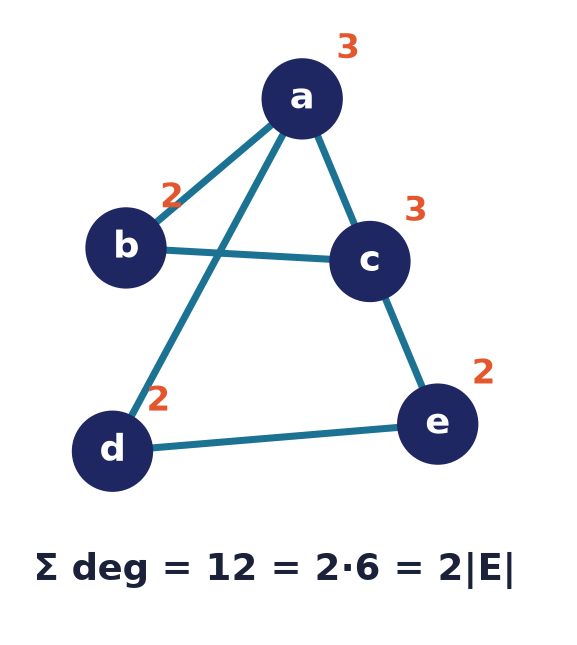
The degree $\deg(v)$ of a vertex is the number of edges incident to it. Because each edge contributes to the degree of exactly two vertices, summing all degrees counts every edge twice — the handshaking theorem:

$$\sum_{v \in V} \deg(v) = 2\,|E|.$$

For the 4-cycle on $\{1,2,3,4\}$ with edges $(1,2),(2,3),(3,4),(4,1)$, every vertex has degree $2$, so the sum is $8 = 2 \cdot 4$. A corollary: the number of vertices of odd degree is always even.

2.3 Matrix representations #

Fix an ordering of the $n$ vertices (and, for incidence, the $m$ edges).

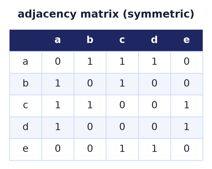
The adjacency matrix $A$ is $n \times n$ with $A[i][j] = 1$ when vertices $i, j$ are adjacent and $0$ otherwise. For an undirected graph it is symmetric. For $V = \{1,2,3\}$, $E = \{(1,2),(2,3)\}$:

      1  2  3
  1 [ 0  1  0 ]
  2 [ 1  0  1 ]
  3 [ 0  1  0 ]

The incidence matrix $M$ is $n \times m$ (vertices $\times$ edges) with $M[v][e] = 1$ when vertex $v$ is an endpoint of edge $e$. For $V = \{A,B,C\}$, $E = \{e_1 = (A,B),\ e_2 = (B,C)\}$:

       e1 e2
  A [  1  0 ]
  B [  1  1 ]
  C [  0  1 ]

Each column of an incidence matrix has exactly two $1$s (its edge’s endpoints).

2.4 Walks, trails, paths, and circuits #

A walk is an alternating sequence of vertices and edges $v_0, e_1, v_1, \dots, e_k, v_k$ where each $e_i = \{v_{i-1}, v_i\}$. Refinements:

• a trail is a walk with no repeated edge;
• a path is a walk with no repeated vertex (hence no repeated edge);
• a circuit (closed trail) is a trail with $v_0 = v_k$; a cycle is a path that returns to its start.

The number of walks between two vertices is generally infinite (edges may be reused), so in practice one enumerates trails or simple paths, which are finite. For $E = \{(1,2),(2,3),(3,4),(4,1)\}$, the sequence $1 \to 2 \to 3 \to 4$ is a path, and $A \to B \to C \to D \to A$ (on the analogous 4-cycle) is a circuit.

2.5 Subgraphs and isomorphism #

$H = (V', E')$ is a subgraph of $G = (V, E)$ if $V' \subseteq V$, $E' \subseteq E$, and every edge of $E'$ joins two vertices of $V'$.

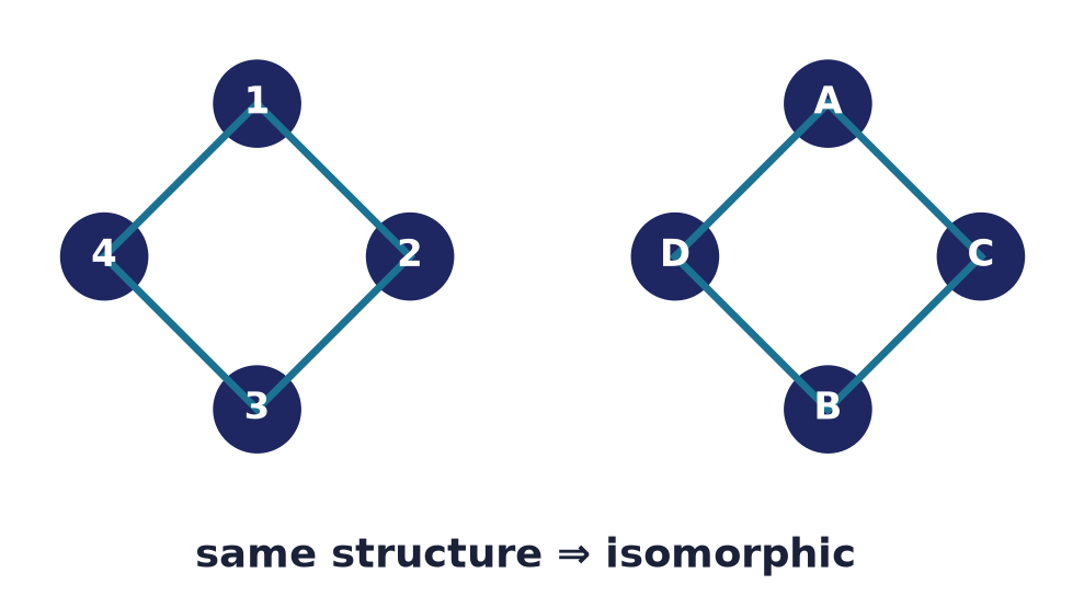
Two graphs $G_1, G_2$ are isomorphic if there is a bijection $f : V_1 \to V_2$ that preserves adjacency: $\{u,v\} \in E_1 \iff \{f(u), f(v)\} \in E_2$. Isomorphic graphs must agree on all invariants — the number of vertices, the number of edges, and the sorted degree sequence — so checking those first quickly rejects most non-isomorphic pairs; a full test then searches for a valid bijection.

2.6 Algorithms #

function degree(V, E, v):
    d ← 0
    for each edge {a, b} in E:
        if a == v or b == v: d ← d + 1
    return d

function adjacencyMatrix(V, E):          # V indexed 0..n-1
    A ← n×n matrix filled with 0
    for each edge {u, v} in E:
        A[idx(u)][idx(v)] ← 1
        A[idx(v)][idx(u)] ← 1
    return A

function incidenceMatrix(V, E):          # n vertices, m edges
    M ← n×m matrix filled with 0
    for j, edge {u, v} in E:             # j = 0 .. m-1
        M[idx(u)][j] ← 1
        M[idx(v)][j] ← 1
    return M

function findPath(V, E, start, goal, visited):   # depth-first search
    add start to visited
    if start == goal: return [start]
    for each w adjacent to start:
        if w not in visited:
            sub ← findPath(V, E, w, goal, visited)
            if sub ≠ null: return [start] + sub
    return null

function findCircuit(V, E):              # a closed trail via DFS back-edge
    depth-first search from each vertex, recording the current trail;
    if an edge leads back to a vertex already on the trail, the segment
    from that vertex to the current one, plus the closing edge, is a circuit.

Subgraph test: confirm $V' \subseteq V$ and, for every edge in $E'$, that the edge is in $E$ and both endpoints are in $V'$.

Isomorphism test: reject immediately if $|V_1|\neq|V_2|$, $|E_1|\neq|E_2|$, or the sorted degree sequences differ; otherwise search for an adjacency-preserving bijection by backtracking (matching vertices of equal degree).

2.7 Complexity #

With $n = |V|$ and $m = |E|$: degree is $O(m)$; building either matrix is $O(n^2)$ (to initialise) plus $O(m)$; findPath (DFS) visits each vertex and edge once, $O(n + m)$. Enumerating all simple paths or trails is exponential in the worst case, and graph isomorphism has no known polynomial-time algorithm — the invariant checks above keep the typical case fast.

Laboratory/Laboratory6/2method.md · 5.4 KB · updated 2026-08-01 18:42