Lecture 4. Boolean algebra — basics
4.1 Overview
This lecture builds the algebraic foundation for the digital‑logic part of the course. We start from the everyday notion of a statement that is either true or false, encode the two truth values as and , and study how statements combine through a small set of logical operations.
The central object is Boolean algebra: the two‑element set with negation (), conjunction () and disjunction (), plus the derived operations exclusive‑or (), implication () and equivalence (). Every operation is completely described by a truth table; a function of Boolean variables is nothing more than a truth table; and these functions obey a compact list of laws — commutativity, associativity, distributivity, De Morgan’s laws, and more. Physical realisation (logic gates), systematic simplification (canonical forms, Karnaugh maps) and the deductive side (propositional logic) come in later lectures; here we stay with the algebra, which — as the final sections show — is literally the same structure you met in set algebra (Lecture 2) and will meet again in propositional logic (Lecture 6).
Why should we care?
Boolean algebra is the mathematics of decisions and yes/no information, and it sits underneath almost everything a computer does.
- Hardware. A wire in a digital circuit is either at a high voltage or a low voltage — two states, exactly the alphabet . A logic gate computes a Boolean operation on its input wires. An adder, a multiplexer, the control unit of a processor — all are Boolean functions realised in silicon. Claude Shannon’s 1937 master’s thesis showed that the algebra Boole invented to formalise reasoning is precisely the algebra of switching circuits, and modern chip design still rests on that identification.
- Software. Every
if,while, and? :in a program is steered by a Boolean expression. The short‑circuit operators&&and||, the bitwise operators& | ~ ^, and the conditions in database queries and search engines (“cats AND (black OR white) NOT kittens”) are Boolean algebra in disguise. - Reasoning. The same laws let us decide when two conditions are equivalent (so one can safely replace the other), when a condition can never be satisfied (a bug — dead code), and when one always holds (a redundant test).
The pay‑off of this lecture is a small toolkit — a dozen laws and one principle (duality) — that lets you transform, simplify and reason about such expressions with the confidence of ordinary algebra.
Roadmap
We proceed from statements to their symbolic encoding; define the elementary operations by truth tables; count how many Boolean functions of variables exist (the answer, , is proved); introduce tautologies, contradictions and logical equivalence; state the laws and prove every one of them by truth table; state and justify the duality principle; show how identities are also derived algebraically; and finally explain in what precise sense logic, sets and bits are three faces of one structure. A short historical note and a list of exercises close the chapter.
4.2 Statements (propositions) and truth values
A statement (or proposition) is a declarative sentence that is either true or false, but not both. Being a statement has nothing to do with our knowing which of the two it is — only with the sentence being definitely one or the other.
Examples and non‑examples.
- “Today is Sunday.” — a statement (true or false depending on the day).
- “.” — a statement (true).
- “There are infinitely many twin primes.” — a statement: it is definitely true or definitely false, even though (as of today) nobody knows which. Having a truth value does not require us to know it.
- “.” — this is a predicate (open sentence): it becomes a statement only once is fixed. Predicates with variables and quantifiers are the subject of predicate logic, not of this lecture.
- “How are you?” — not a statement; a question has no truth value.
- “Close the door.” — not a statement; a command has no truth value.
- “This sentence is false.” — not a statement; assuming it true makes it false and vice versa, so it can be assigned neither value consistently (the liar paradox).
We attach a symbolic truth value to every statement:
Working with the digits and (rather than the words) is exactly what turns logic into an algebra: truth values become quantities we can compute with, and logical connectives become operations like and .
Remark. Some authors write , some , some . This course uses and almost everywhere, because it makes the bridge to arithmetic and hardware immediate: conjunction will behave exactly like multiplication of bits, and disjunction almost like addition.
Compound statements
Simple statements are usually named by letters and combined into compound statements using connectives. Let
- = “Today is Friday”,
- = “The weather is good”.
Then:
| Compound statement | Reads as |
|---|---|
| “Today is Friday and the weather is good” | |
| “Today is Friday or the weather is good” | |
| “Today is not Friday” | |
| “Today is not Friday and the weather is good” |
The truth value of a compound statement depends only on the truth values of its parts and on the connectives used — never on the meaning of the words. This property is called truth‑functionality, and it is the whole point of moving to Boolean algebra: once the parts’ truth values are fixed, the compound’s value is determined by pure calculation.
4.3 Elementary logical operations
The alphabet of Boolean algebra is just the two symbols . On top of it we define the operations below. Each operation is defined by a truth table that lists its output for every combination of inputs. We list input rows in ascending binary order (); other authors use a different row order, but the operation is the same.
Negation (NOT, )
Negation flips the truth value: is true exactly when is false. Common notations: , , , , . Negation is a unary operation (one input); all the others below are binary (two inputs).
| 0 | 1 |
| 1 | 0 |
Conjunction (AND, )
Conjunction is true exactly when both operands are true. Notations: , , . Comparing the table below with a multiplication table for shows they are identical: . This is why conjunction is often written as a product.
| 0 | 0 | 0 |
| 0 | 1 | 0 |
| 1 | 0 | 0 |
| 1 | 1 | 1 |
Disjunction (OR, )
Disjunction is true when at least one operand is true (this is the inclusive or). Notations: , . It behaves like addition of bits except that (not ): disjunction is “saturating” addition capped at .
| 0 | 0 | 0 |
| 0 | 1 | 1 |
| 1 | 0 | 1 |
| 1 | 1 | 1 |
Common pitfall. Everyday English “or” is often exclusive (“soup or salad” means one, not both), but the logical is inclusive: . The exclusive reading is a different operation, XOR, defined next.
Exclusive‑or (XOR, )
Exclusive‑or is true when the operands differ — exactly one of them is true. It is the “or, but not both” of everyday speech, and also “the operands are unequal”, so iff . It behaves like addition modulo 2: .
| 0 | 0 | 0 |
| 0 | 1 | 1 |
| 1 | 0 | 1 |
| 1 | 1 | 0 |
Because is addition mod 2 it has a clean algebra: , , ; it is commutative and associative; and distributes over it, . This makes a field, and is the basis of the algebraic normal form (Lecture 5) and of parity/checksum circuits.
Implication (IF … THEN …, )
Implication (“if then ”) is false in only one case: a true premise leading to a false conclusion . In particular, whenever is false the implication is vacuously true — a false premise never breaks a promise. Here is the antecedent (hypothesis) and the consequent (conclusion). Notations: , , .
| 0 | 0 | 1 |
| 0 | 1 | 1 |
| 1 | 0 | 0 |
| 1 | 1 | 1 |
Think of as the promise “if happens, then I guarantee ”. The promise is broken only if happens and fails to — the single row.
Common pitfall. Implication is not symmetric: and are different functions (compare their columns). And is not ; the correct negation is (the promise is broken exactly when the premise holds but the conclusion fails). Also, carries no idea of cause: “If then the moon is cheese” is true, because the premise is false.
Equivalence (IF AND ONLY IF, )
Equivalence (also written or ) is true when both operands have the same truth value. It is exactly the negation of XOR: , i.e. iff .
| 0 | 0 | 1 |
| 0 | 1 | 0 |
| 1 | 0 | 0 |
| 1 | 1 | 1 |
All binary operations at a glance
Putting the two‑variable operations side by side makes their patterns easy to compare:
| 0 | 0 | 0 | 0 | 0 | 1 | 1 |
| 0 | 1 | 0 | 1 | 1 | 1 | 0 |
| 1 | 0 | 0 | 1 | 1 | 0 | 0 |
| 1 | 1 | 1 | 1 | 0 | 1 | 1 |
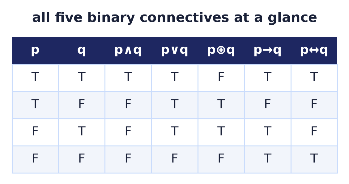
Only three of these operations are primitive; the rest are abbreviations. We will prove below (and again in Lecture 5) that , and can each be rewritten with , , alone. Two identities worth memorising now, because they are used constantly, are
The first is verified in the worked examples below.
4.4 Precedence and reading compound expressions
To avoid a thicket of parentheses we adopt the standard precedence (binding strength), from tightest to loosest:
Thus means , and means , and means . Negation applies to the smallest expression to its right; binds like multiplication and like addition. When in doubt, parenthesise: clarity beats brevity.
Common pitfall. is , not — the bar/¬ does not stretch over the unless you write it that way. In the notation vs the difference is visible; in linear text it is a frequent source of error.
4.5 Boolean variables and Boolean functions
A Boolean variable is a variable that ranges over . A Boolean function of variables is any rule
that assigns a value or to each of the possible input combinations. Here is the set of all ‑tuples (input vectors) of bits.
A truth table is the function. Because the domain is finite, a Boolean function is fully specified simply by listing its output on every input row. Two Boolean expressions denote the same function precisely when their truth tables agree in every row. This is the single most important tool of the chapter:
To prove that two Boolean expressions are equal, build both truth tables and check that the final columns are identical, row by row. To disprove equality, it is enough to exhibit one row where they differ (a counterexample).
Counting Boolean functions
How many different Boolean functions of variables are there? The answer is surprisingly large and grows doubly exponentially.
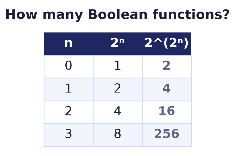
Theorem (number of Boolean functions). The number of Boolean functions of variables is
Proof. We count in two stages.
Stage 1 — the number of input rows. An input is an ‑tuple with each . By the multiplication (product) rule there are independent choices for each of the coordinates, so
distinct input rows. Call this number .
Stage 2 — the number of ways to fill the output column. A function is determined exactly by the value assigns to each of the input rows, and these values may be chosen independently: any of the output columns of length (each entry or ) determines a genuine function, and different columns determine different functions (they differ on some row). Again by the product rule there are
such columns. Substituting gives .
The two‑stage structure — first count the rows , then count the fillings — is the reason the exponent is itself an exponential.
| rows | functions | |
|---|---|---|
| 0 | 1 | 2 |
| 1 | 2 | 4 |
| 2 | 4 | 16 |
| 3 | 8 | 256 |
| 4 | 16 | 65 536 |
| 5 | 32 | 4 294 967 296 |
The growth is ferocious: already at there are functions, more than the number of grains of sand on Earth. This explosion is exactly why systematic simplification methods (Lecture 5) are needed — one cannot search all functions by hand.
The case . A function of no variables has the single empty input tuple as its only “row” ( row), and there are such functions: the constant and the constant . This matches the two truth values and is a good sanity check on the formula.
Example — the 4 functions of one variable. For the theorem gives :
| 0 | 0 | 0 | 1 | 1 |
| 1 | 0 | 1 | 0 | 1 |
They are: the constant , the identity , the negation , and the constant . There are literally no others — every possible two‑row output column appears.
Example — the 16 functions of two variables. With there are exactly functions . Reading each column top‑to‑bottom over the input rows gives its truth table (and the subscript is the binary number spelled by that column, MSB at the top):
| 0 | 0 | 0 | 0 | 0 | 0 | 0 | 0 | 0 | 0 | 1 | 1 | 1 | 1 | 1 | 1 | 1 | 1 |
| 0 | 1 | 0 | 0 | 0 | 0 | 1 | 1 | 1 | 1 | 0 | 0 | 0 | 0 | 1 | 1 | 1 | 1 |
| 1 | 0 | 0 | 0 | 1 | 1 | 0 | 0 | 1 | 1 | 0 | 0 | 1 | 1 | 0 | 0 | 1 | 1 |
| 1 | 1 | 0 | 1 | 0 | 1 | 0 | 1 | 0 | 1 | 0 | 1 | 0 | 1 | 0 | 1 | 0 | 1 |
Several of these columns are the operations we already named:
- (constant false), (constant true);
- (AND), (OR);
- , , , (projections and their negations);
- (XOR), (equivalence);
- , (implications);
- (NOR), (NAND).
The important takeaway is not the individual names but the count: every possible two‑variable truth table appears exactly once, and there are of them — no more, no fewer. (The exhaustive named list of these sixteen, and how NAND or NOR alone can generate them all, is taken up in Lecture 5.)
4.6 Truth tables of compound expressions
Any compound expression is evaluated column by column: introduce a helper column for each sub‑expression, fill it from the operator’s truth table, and combine helper columns until the final column is reached. With variables the table has rows. List the rows in ascending binary order so that nothing is skipped.
Example 1 (easy) — evaluate . Two rows suffice, and the result recovers :
| 0 | 1 | 0 |
| 1 | 0 | 1 |
The final column equals the column: . (This is the involution law, proved formally below.)
Example 2 (easy) — evaluate . Three variables give rows. Build , then , then their disjunction:
| 0 | 0 | 0 | 0 | 1 | 1 |
| 0 | 0 | 1 | 0 | 0 | 0 |
| 0 | 1 | 0 | 0 | 1 | 1 |
| 0 | 1 | 1 | 0 | 0 | 0 |
| 1 | 0 | 0 | 0 | 1 | 1 |
| 1 | 0 | 1 | 0 | 0 | 0 |
| 1 | 1 | 0 | 1 | 1 | 1 |
| 1 | 1 | 1 | 1 | 0 | 1 |
The last column is the function computed by the expression; it equals on five of the eight rows.
Example 3 (medium) — “exactly one of ”: evaluate .
| 0 | 0 | 0 | 0 | 1 | 0 |
| 0 | 1 | 1 | 0 | 1 | 1 |
| 1 | 0 | 1 | 0 | 1 | 1 |
| 1 | 1 | 1 | 1 | 0 | 0 |
The final column reads — exactly the XOR table. So we have derived the identity , showing that XOR is not a new primitive but a combination of , and .
Example 4 (medium) — equals . This rewriting of implication in terms of the three primitives is used everywhere; here is its proof.
| 0 | 0 | 1 | 1 | 1 |
| 0 | 1 | 1 | 1 | 1 |
| 1 | 0 | 0 | 0 | 0 |
| 1 | 1 | 1 | 0 | 1 |
The columns for and are identical, so .
Example 5 (harder) — the hypothetical syllogism is a tautology. We show that is true in every row — the formal content of “if implies and implies , then implies ”.
| whole formula | |||||||
|---|---|---|---|---|---|---|---|
| 0 | 0 | 0 | 1 | 1 | 1 | 1 | 1 |
| 0 | 0 | 1 | 1 | 1 | 1 | 1 | 1 |
| 0 | 1 | 0 | 1 | 0 | 0 | 1 | 1 |
| 0 | 1 | 1 | 1 | 1 | 1 | 1 | 1 |
| 1 | 0 | 0 | 0 | 1 | 0 | 0 | 1 |
| 1 | 0 | 1 | 0 | 1 | 0 | 1 | 1 |
| 1 | 1 | 0 | 1 | 0 | 0 | 0 | 1 |
| 1 | 1 | 1 | 1 | 1 | 1 | 1 | 1 |
The final column is all $1$s, so the formula is a tautology. Notice the mechanism: on every row where the hypothesis is (rows ), the conclusion is also ; on the remaining rows the hypothesis is , so the outer implication is vacuously .
4.7 Tautologies, contradictions, and logical equivalence
A tautology is an expression whose value is for every assignment of its variables — the final truth‑table column is all $1$s. A contradiction (or unsatisfiable expression) is an expression whose value is for every assignment — the final column is all $0$s. An expression that is on at least one row is called satisfiable; one that is on some rows and on others is a contingency.
Example — the tautology (the law of excluded middle):
| 0 | 1 | 1 |
| 1 | 0 | 1 |
Example — the contradiction (the law of non‑contradiction):
| 0 | 1 | 0 |
| 1 | 0 | 0 |
These two facts, and , are the complement laws and appear among the axioms below.
Logical equivalence. Two expressions and are logically equivalent, written , when they have the same truth value in every row — equivalently, when the biconditional is a tautology. This is the precise meaning of the “” sign in every Boolean identity: is . So the whole next section is a catalogue of logical equivalences, each certified by a truth table.
Remark. Satisfiability — “is there an assignment making this expression ?” — is the celebrated SAT problem, the first problem proved NP‑complete (Cook, 1971). A truth table settles it in rows, but for large that is hopeless, which is why SAT is central to complexity theory. We only need the small‑ case here.
4.8 The laws (identities) of Boolean algebra
The following identities hold for all Boolean variables. They are written in dual pairs: an AND‑form and an OR‑form.
| Law | AND‑form () | OR‑form () |
|---|---|---|
| Commutative | ||
| Associative | ||
| Distributive | ||
| Identity | ||
| Domination | ||
| Idempotent | ||
| Complement | ||
| Absorption | ||
| De Morgan | ||
| Involution | (self‑dual) |
We now prove each law by the truth‑table method: build both sides and compare final columns. Since means precisely “same value in every row”, a matching pair of columns is a complete proof.
Commutativity
Theorem. and .
Proof. All four rows for both operations:
| 0 | 0 | 0 | 0 | 0 | 0 |
| 0 | 1 | 0 | 0 | 1 | 1 |
| 1 | 0 | 0 | 0 | 1 | 1 |
| 1 | 1 | 1 | 1 | 1 | 1 |
Column equals column , and column equals column , in every row.
Associativity
Theorem. and .
Proof. For conjunction:
| 0 | 0 | 0 | 0 | 0 | 0 | 0 |
| 0 | 0 | 1 | 0 | 0 | 0 | 0 |
| 0 | 1 | 0 | 0 | 0 | 0 | 0 |
| 0 | 1 | 1 | 0 | 0 | 1 | 0 |
| 1 | 0 | 0 | 0 | 0 | 0 | 0 |
| 1 | 0 | 1 | 0 | 0 | 0 | 0 |
| 1 | 1 | 0 | 1 | 0 | 0 | 0 |
| 1 | 1 | 1 | 1 | 1 | 1 | 1 |
The columns and agree (both are exactly when ). For disjunction:
| 0 | 0 | 0 | 0 | 0 | 0 | 0 |
| 0 | 0 | 1 | 0 | 1 | 1 | 1 |
| 0 | 1 | 0 | 1 | 1 | 1 | 1 |
| 0 | 1 | 1 | 1 | 1 | 1 | 1 |
| 1 | 0 | 0 | 1 | 1 | 0 | 1 |
| 1 | 0 | 1 | 1 | 1 | 1 | 1 |
| 1 | 1 | 0 | 1 | 1 | 1 | 1 |
| 1 | 1 | 1 | 1 | 1 | 1 | 1 |
The columns and agree (both are exactly when ).
Remark. Associativity is what lets us write and without parentheses at all: the grouping does not affect the value. Together with commutativity it means a long AND (resp. OR) is just “are all inputs ?” (resp. “is at least one input ?”), regardless of order or grouping.
Distributivity
Theorem. and .
Proof. First form ( over ):
| 0 | 0 | 0 | 0 | 0 | 0 | 0 | 0 |
| 0 | 0 | 1 | 1 | 0 | 0 | 0 | 0 |
| 0 | 1 | 0 | 1 | 0 | 0 | 0 | 0 |
| 0 | 1 | 1 | 1 | 0 | 0 | 0 | 0 |
| 1 | 0 | 0 | 0 | 0 | 0 | 0 | 0 |
| 1 | 0 | 1 | 1 | 1 | 0 | 1 | 1 |
| 1 | 1 | 0 | 1 | 1 | 1 | 0 | 1 |
| 1 | 1 | 1 | 1 | 1 | 1 | 1 | 1 |
The columns and coincide. Second form ( over ):
| 0 | 0 | 0 | 0 | 0 | 0 | 0 | 0 |
| 0 | 0 | 1 | 0 | 0 | 0 | 1 | 0 |
| 0 | 1 | 0 | 0 | 0 | 1 | 0 | 0 |
| 0 | 1 | 1 | 1 | 1 | 1 | 1 | 1 |
| 1 | 0 | 0 | 0 | 1 | 1 | 1 | 1 |
| 1 | 0 | 1 | 0 | 1 | 1 | 1 | 1 |
| 1 | 1 | 0 | 0 | 1 | 1 | 1 | 1 |
| 1 | 1 | 1 | 1 | 1 | 1 | 1 | 1 |
The columns and coincide.
Remark. The first form mimics ordinary arithmetic (). The second form, , has no analogue in ordinary arithmetic — in general — and is a hallmark of Boolean algebra. In Boolean algebra, and distribute over each other, perfectly symmetrically.
Identity and domination
Theorem. , (identity); , (domination).
Proof. Here and are constants, so only the two values of matter:
| 0 | 0 | 0 | 0 | 1 |
| 1 | 1 | 1 | 0 | 1 |
Columns and equal the column; column is constantly ; column is constantly .
The identity law says is the neutral element for and is the neutral element for (compare and ). Domination says annihilates under (like ) and annihilates under .
Idempotence
Theorem. and .
Proof.
| 0 | 0 | 0 |
| 1 | 1 | 1 |
Both columns equal .
Remark. Idempotence is where Boolean algebra departs sharply from arithmetic: and hold for all Boolean values, whereas and are usually different from . Consequently repeated terms collapse — — which is the first tool of simplification.
Complement
Theorem. and .
Proof.
| 0 | 1 | 0 | 1 |
| 1 | 0 | 0 | 1 |
Column is constantly ; column is constantly .
These are exactly the contradiction and the tautology met earlier: a value and its negation can never both hold, and one of them always holds.
Involution
Theorem. .
Proof.
| 0 | 1 | 0 |
| 1 | 0 | 1 |
The column equals the column.
Involution is self‑dual: swapping and leaves it unchanged, since it mentions neither.
Absorption
Theorem. and .
Proof. First form:
| 0 | 0 | 0 | 0 |
| 0 | 1 | 1 | 0 |
| 1 | 0 | 1 | 1 |
| 1 | 1 | 1 | 1 |
Column equals the column. Second form:
| 0 | 0 | 0 | 0 |
| 0 | 1 | 0 | 0 |
| 1 | 0 | 0 | 1 |
| 1 | 1 | 1 | 1 |
Column equals the column.
Remark. “Absorption” names the phenomenon that the term is swallowed whole: whatever is, it makes no difference. Circuit designers love absorption because it deletes an entire gate. An algebraic derivation (not a truth table) is given in the next section.
De Morgan’s laws
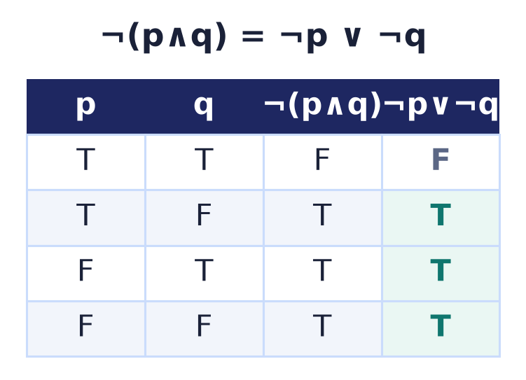
Theorem (De Morgan). and .
Proof. First law:
| 0 | 0 | 0 | 1 | 1 | 1 | 1 |
| 0 | 1 | 0 | 1 | 1 | 0 | 1 |
| 1 | 0 | 0 | 1 | 0 | 1 | 1 |
| 1 | 1 | 1 | 0 | 0 | 0 | 0 |
The columns and are equal in every row. Second law:
| 0 | 0 | 0 | 1 | 1 | 1 | 1 |
| 0 | 1 | 1 | 0 | 1 | 0 | 0 |
| 1 | 0 | 1 | 0 | 0 | 1 | 0 |
| 1 | 1 | 1 | 0 | 0 | 0 | 0 |
The columns and are equal in every row.
Common pitfall. De Morgan’s laws say the negation flips the connective: is , not . “Not (rich and famous)” means “poor or obscure”, not “poor and obscure”. Distributing a negation across / without switching the connective is the single most common error in this subject. In hardware terms: NOT of an AND is an OR of NOTs (a NAND rearranges into an OR gate with inverted inputs), and dually for NOR.
De Morgan’s laws also show that and each suffice to express the other connective: and . This idea of a functionally complete set of operations is developed fully in Lecture 5.
4.9 The duality principle
Look again at the table of laws: the two columns are mirror images. Swap and throughout, and every left‑hand identity becomes the right‑hand one. This is no coincidence.
The dual of an expression. Given a Boolean expression built from variables, the constants , and the operations , its dual is obtained by interchanging and everywhere, while leaving variables and negations untouched. For instance the dual of is .
Duality Principle. If an identity holds for all Boolean values, then the dual identity also holds.
The practical consequence is that the laws come in pairs for free: prove one form and its dual is automatically a theorem. This halves the work of building and memorising the theory. But why is it true? The justification rests on De Morgan and involution.
Lemma (complementation is dualization with negated inputs). For every Boolean expression built from and constants,
as functions.
Proof. By structural induction on the way is built.
Base cases.
- (a variable). Then , so . ✓
- . Then , and . ✓
- . Then , and . ✓
Inductive step. Assume the claim for sub‑expressions .
- . Then , and
- . Dually, and . ✓
- . Negation is unchanged by dualization, so , and
So . ✓
By induction the identity holds for every expression .
Proof of the Duality Principle. Suppose holds for all inputs. Then holds for all inputs as well. By the Lemma,
As ranges over all of , the negated tuple also ranges over all of (negation is a bijection of ). Hence for all , i.e. .
Example. The distributive law has dual — the second distributive law, which we no longer need to prove separately. Likewise absorption dualizes to , and the two De Morgan laws are duals of each other.
Common pitfall. The dual is not the negation. To dualize you swap and but leave the variables and their bars alone. Negating an expression is a different operation (and, by the Lemma above, equals the dual only after you also negate every variable).
4.10 Proving identities algebraically
Truth tables always work, but for expressions with many variables they are long. Once the laws are established, we can also prove new identities algebraically — by rewriting one side into the other using the laws as rewrite rules. This is exactly how one simplifies circuits (Lecture 5), and it is the style of proof used in propositional logic (Lecture 6).
Example — absorption derived from the axioms. We prove using only identity, distributivity and domination:
By the duality principle, dualizing every step proves the other absorption law at once — no separate calculation required.
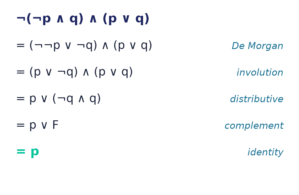
Example — simplify .
A four‑operator expression collapses to the single variable . Verifying this by truth table would take four rows; the algebra explains why it holds.
Remark. An algebraic proof and a truth‑table proof establish the same fact but serve different purposes. The truth table is a decision procedure — it always terminates with a yes/no. The algebraic derivation gives insight and structure, and it scales to symbolic settings where truth tables do not (e.g. reasoning about circuits with hundreds of inputs, where rows is out of reach).
4.11 Three faces of one structure: logic, sets, and bits
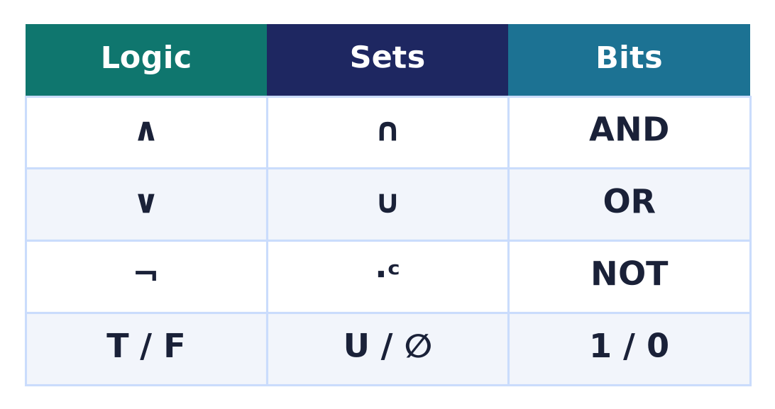
The laws we proved are not special to truth values. The same list of laws governs the algebra of sets (Lecture 2) and the algebra of propositions (Lecture 6). This is because all three are instances of one abstract structure — a Boolean algebra — and we can line the three up operation for operation.
| Concept | Propositional logic | Set algebra | Boolean (bit) algebra |
|---|---|---|---|
| “or” | |||
| “and” | |||
| “not” | |||
| bottom / empty | (contradiction) | ||
| top / universe | (tautology) | ||
| “same” | |||
| “at most” |
Every law reads identically down any column. For example, De Morgan appears as
and absorption, distributivity, complement, and the rest all match line for line. This is why a fact proved in one setting transfers to the others; the membership table you used for sets in Lecture 2 is the same computation as the truth table you use here.
A genuine isomorphism (sets bit vectors). The correspondence between sets and bits can be made completely precise. Fix a universe . To each subset associate its characteristic (indicator) function
The map is a bijection between the power set and the set of all bit‑valued functions on (both have elements, and the map is clearly one‑to‑one and onto). Moreover it respects every operation, computed pointwise:
A structure‑preserving bijection like this is called an isomorphism: set algebra on is, up to renaming, the coordinatewise Boolean algebra . In the smallest case we get exactly — the two‑element bit algebra of this lecture, with and .
And propositional logic. On the logic side, formulas modulo logical equivalence (grouping together all formulas with the same truth table) form a Boolean algebra too, with as operations, the class of contradictions as , and the class of tautologies as . So the three “faces” are:
- bits under — the hardware/arithmetic view;
- subsets of a universe under — the set view;
- propositions (up to equivalence) under and/or/not — the reasoning view.
They obey the same laws because they are the same algebra wearing three costumes. This is the deep reason the Venn‑diagram intuition from Lecture 2 and the truth tables of this lecture never conflict.
4.12 A note on history: Boole and Shannon
The algebra of this chapter is named for George Boole (1815–1864), a largely self‑taught English mathematician. In The Mathematical Analysis of Logic (1847) and the fuller An Investigation of the Laws of Thought (1854), Boole argued that the laws of correct reasoning could be written as algebraic equations over quantities taking the values and — turning logic, for the first time, into calculation. The idempotent law (our ) was, in Boole’s own treatment, the equation that singled out this special algebra from ordinary algebra.
The bridge to computing came much later. In his 1937 MIT master’s thesis, A Symbolic Analysis of Relay and Switching Circuits, Claude Shannon (1916–2001) observed that a network of on/off switches obeys exactly Boole’s laws — a switch is or , series wiring is , parallel wiring is — so any switching circuit can be designed and simplified algebraically. That single insight is the theoretical foundation of all digital hardware. It is often called one of the most influential master’s theses ever written.
4.13 Connections to computer science and hardware
Boolean algebra is the working mathematics of the machine layer. A few threads we will pick up or that you already use:
- Logic gates. The primitive operations (and the derived NAND, NOR, XOR) are realised as physical gates; a Boolean expression becomes a circuit and vice versa. Lecture 5 builds gates, translates expressions to circuits, and shows how NAND or NOR alone can implement everything.
- Minimization. Because there are functions but many expressions for each, we want the smallest expression (fewest gates). The laws above — especially absorption, distributivity and idempotence — are the algebraic tools; canonical normal forms (CDNF/CCNF) and Karnaugh maps are the systematic ones, both in Lecture 5.
- Bitwise operations. In C/Java/Python the operators
&,|,~,^apply to all bits of an integer in parallel — Boolean algebra on or independent copies at once. Masks, flags and toggles are De Morgan and complement in action. - Control flow and short‑circuiting.
&&and||evaluate left‑to‑right and stop early; their algebra is exactly and , and refactoring a condition safely (e.g.!(a && b)into!a || !b) is De Morgan. - Search and databases. Query languages combine conditions with AND/OR/NOT; query optimisation rewrites them using these very laws.
- Deductive logic. The tautologies and equivalences here become the propositional equivalences of Lecture 6 (propositional logic) and the rules of inference of Lecture 7 (proof techniques) — for instance, the hypothetical syllogism proved above.
Chapter summary
- A statement is a declarative sentence that is definitely true or false; we encode the values as (true) and (false). Compound statements are truth‑functional: their value depends only on the parts’ values and the connectives.
- Boolean algebra works over the alphabet with the primitive operations and the derived operations ; each is defined by a truth table. Standard precedence is .
- is true only when both inputs are ; (inclusive) is true when at least one is ; is true when the inputs differ; is false only for ; is true when the inputs match. Key rewrites: and .
- A Boolean function of variables is exactly a truth table with rows; there are such functions ( for , for , for , for ) — proved by counting rows then fillings.
- A tautology is always ; a contradiction is always ; expressions are logically equivalent () when their columns match, which is what a Boolean identity means. Compound expressions are evaluated column by column.
- The laws (commutative, associative, distributive, identity, domination, idempotent, complement, absorption, involution, De Morgan) come in dual pairs and were each proved by truth table. Identities can also be derived algebraically from the laws.
- The Duality Principle — swap and — turns any true identity into another true identity; it is justified via the lemma , proved by structural induction from De Morgan and involution.
- Logic, sets and bits are one structure. , , complement, , ; the characteristic‑function map is a genuine isomorphism , so every law transfers among the three.
- Forward pointers: gates, functional completeness, canonical forms and Karnaugh maps in Lecture 5; the semantics of propositional logic in Lecture 6; proof and inference in Lecture 7.
Exercises
Warm‑up
-
Statement or not? Classify each sentence as a statement (proposition) or not, and if it is a statement give its truth value where possible: (a) “ is prime.” (b) “Read Lecture 4.” (c) “.” (d) “Every even number greater than is a sum of two primes.” (e) “Ouch!”
-
Fill the tables. From memory, write the truth tables of , , , , , . State in one phrase what makes each operation output .
-
Evaluate at a point. With , , , compute the value of and of .
-
Precedence. Insert full parentheses according to the standard precedence: (a) (b) (c) .
-
When is it false? State the single row on which is , and explain in words why is whenever .
-
Dictionary. Give the set‑algebra counterpart and the propositional‑logic counterpart of each of , , , , .
Standard
-
Build a table. Construct the full truth table of and state on how many of the rows it equals .
-
Implication rewrite. Prove by truth table, then use it to write in terms of and only.
-
Contrapositive. Prove by truth table that . (This equivalence is the basis of proof by contraposition, Lecture 7.)
-
Second De Morgan. Prove by constructing and comparing truth tables.
-
Both absorptions. Verify by truth table, then give a purely algebraic derivation of from the laws.
-
XOR in primitives. Show by truth table.
-
Classify. For each formula decide whether it is a tautology, a contradiction, or a contingency, and justify with its final column: (a) (b) (c) (d) .
-
Duals. Write the dual of each identity (do not negate): (a) (b) (c) .
-
Counting. How many Boolean functions are there of variables? Of variables? Of the two‑variable functions, how many are commutative (satisfy )? Justify the last count.
-
Simplify algebraically. Using the laws, simplify and to a single variable each. Name every law you use.
Challenge
-
Hypothetical syllogism. Prove that is a tautology, and identify which rows make the outer implication vacuously true.
-
Duality by hand. For the specific expression , write down , and verify the lemma by an ‑row truth table.
-
Self‑dual functions. A Boolean function is self‑dual if , equivalently for all inputs. How many self‑dual functions of variables are there? (Hint: pair each input with its bitwise complement.) List one non‑trivial example.
-
Isomorphism check. Let , , . Write the characteristic vectors (order the coordinates ). Compute , and coordinatewise, and confirm they are the characteristic vectors of , and respectively.
Selected answers & hints
1. (a) statement, true. (b) not a statement (command). (c) open sentence — a statement only once is fixed. (d) statement (Goldbach’s conjecture): it has a definite truth value even though it is currently unknown. (e) not a statement (exclamation).
3. . .
4. (a) . (b) . (c) .
5. False only on the row . When the promise “if then ” is never triggered, so it cannot be broken — the implication is vacuously .
7. The column of is on exactly of the rows — those with and , namely .
8. The two columns match (see Example 4). Then by De Morgan and involution.
9. Both columns equal over the rows ; hence equivalent.
11. Table for reads . Algebraic derivation of the dual: (identity, distributive, domination, identity) — or simply dualize the derivation in the text.
13. (a) tautology; (b) tautology (a contradiction implies anything); (c) contradiction; (d) contradiction (it asserts together with and , which is impossible).
14. (a) . (b) . (c) .
15. variables: . variables: . Commutative two‑variable functions: the outputs on rows and must be equal, so we freely choose the output on row ( ways), on the merged ( ways) and on row ( ways): .
16. (distributive, complement, identity). (dual distributive, complement, identity).
17. See the worked ‑row table in the text; the final column is all $1$s. The outer implication is vacuously true on exactly the rows where the hypothesis is , namely .
18. , with column over , so has column . Dually , and , whose column is also . The two columns agree in all four rows, confirming .
19. self‑dual functions of two variables. The inputs pair up as and under bitwise complement; on each pair the two outputs must be complementary, leaving pairs choices . Example: the projection is self‑dual.
20. , . Then with ; with ; with . All three match, illustrating the isomorphism.
Further reading
- K. H. Rosen, Discrete Mathematics and Its Applications — the chapter on logic and logical equivalences (propositional logic, laws, tautologies) and the chapter on Boolean algebra (Boolean functions, identities, duality, gates).
- S. S. Epp, Discrete Mathematics with Applications — the chapter on the logic of compound statements (truth tables, logical equivalence, De Morgan’s laws) and the section on Boolean algebras and digital logic circuits.
- Historical primary sources: G. Boole, An Investigation of the Laws of Thought (1854); C. E. Shannon, “A Symbolic Analysis of Relay and Switching Circuits” (1938).