2. Methodical guidelines / Методичні вказівки #

This section is self-contained: it collects the counting principles and the basic probability rules needed for the theme, together with the techniques used to solve the tasks in 3classroom.md. For fuller treatment see Lecture 13.

2.1 The two counting principles #

• Product rule (multiplication). If a procedure is a sequence of $k$ independent steps with $n_1, n_2, \dots, n_k$ choices, the whole procedure has $n_1\cdot n_2\cdots n_k$ outcomes. (“And / in stages” $\Rightarrow$ multiply.)
• Sum rule (addition). If an object comes from one of several disjoint cases with $m_1, m_2, \dots$ options, the total is $m_1+m_2+\cdots$. (“Or / separate cases” $\Rightarrow$ add.)

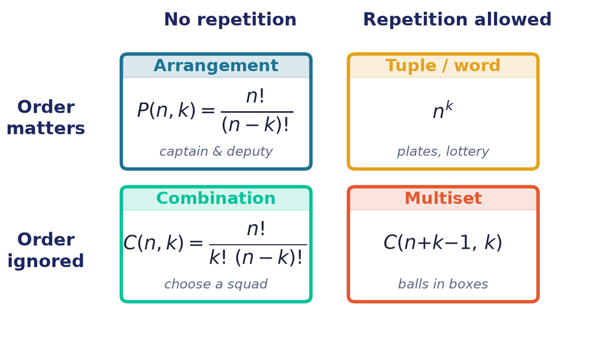
Everything below is the product rule applied to a selection of $k$ objects from $n$, sorted by two yes/no questions: does order matter? and is repetition allowed?

2.2 Order matters — arrangements and tuples #

• With repetition (a tuple / “word”). Each of the $k$ positions is filled independently from $n$ symbols, so there are $\ n^{k}\$ outcomes. (A $4$-letter, $12$-symbol code has $12^4$ possibilities.)
• Without repetition (an arrangement, a $k$-permutation). The first position has $n$ choices, the next $n-1$, and so on for $k$ factors:

$$P(n,k)=\frac{n!}{(n-k)!}=n(n-1)\cdots(n-k+1).$$

A full arrangement ($k=n$) is a permutation: $P(n,n)=n!$.

2.3 Order ignored — combinations and multisets #

• Without repetition (a combination, a subset). A $k$-element subset of $n$ objects; since the $k!$ orders of one subset are now the same, divide the arrangement count by $k!$:

$$C(n,k)=\binom{n}{k}=\frac{P(n,k)}{k!}=\frac{n!}{k!\,(n-k)!}.$$

• With repetition (a multiset). Choosing $k$ objects from $n$ types with repetition allowed — equivalently, distributing $k$ identical balls into $n$ distinct boxes — is counted by stars and bars: line up $k$ stars and $n-1$ bars, so

$$\overline{C}(n,k)=\binom{n+k-1}{k}.$$

(Stars and bars, one of the counting tools from L13; the picture is $k$ stars split into $n$ groups by $n-1$ bars, e.g. $\star\star|\;|\star$ puts $2,0,1$ balls in three boxes.)

The four cases together:

2.4 Classical (Laplace) probability #

When a random experiment has a finite set $\Omega$ of equally likely outcomes, the probability of an event $A\subseteq\Omega$ is

$$P(A)=\frac{|A|}{|\Omega|}=\frac{\text{favourable outcomes}}{\text{all outcomes}}, \qquad 0\le P(A)\le 1.$$

So a probability is a counting problem: count the favourable outcomes (numerator) and all outcomes (denominator), each with the combinatorics of §2.2–2.3. The complement rule is often the shortcut for “at least one”:

$$P(\overline{A})=1-P(A)\quad\Longrightarrow\quad P(\text{at least one})=1-P(\text{none}).$$

2.5 Combining events — independence and conditioning #

• Independent events (one does not affect the other, e.g. draws from different boxes): $\ P(A\cap B)=P(A)\cdot P(B)$. This extends the product rule to probabilities.
• Conditional probability — the probability of $A$ given that $B$ happened — is $P(A\mid B)=\dfrac{P(A\cap B)}{P(B)}$, which rearranges to the multiplication rule $\ P(A\cap B)=P(B)\,P(A\mid B)$. Use it when the population is described in stages (“$96\%$ are good; of the good, $75\%$ are first grade”).
• Drawing several without replacement is handled either by combinations — $P=\dfrac{C(\text{favourable})}{C(\text{total})}$ — or by the multiplication rule with shrinking counts: $\dfrac{10}{24}\cdot\dfrac{9}{23}$ for two whites in a row.

2.6 Working checklist #

• Counting. Ask order? and repetition? and read the formula off §2.3’s chart: $n^k$, $P(n,k)$, $C(n,k)$, or $\binom{n+k-1}{k}$. Independent stages (colours, ranks) multiply.
• Probability. For equally-likely outcomes, count favourable over total. Draws from different sources multiply ($P(A)P(B)$); several from the same source without replacement use combinations or shrinking fractions.
• “At least one”. Take the complement: $1-P(\text{none})$.
• Staged populations. Multiply along the branch: $P(\text{good})\cdot P(\text{1st}\mid\text{good})$.

Practical/Practical6/2method.md · 4.4 KB · updated 2026-08-01 20:18