Lecture 2. Set algebra
Overview
Lecture 1 introduced what a set is: an unordered collection of distinct objects, compared by the subset relation and measured by cardinality. This lecture is about what we do with sets — how to combine and transform them, and, crucially, which algebraic laws these operations obey.
The payoff is twofold. First, we obtain a small toolkit of operations (union, intersection, difference, symmetric difference, complement) that let us build new sets from old ones. Second — and this is the heart of the chapter — these operations satisfy a fixed collection of identities that make set expressions manipulable symbolically, exactly the way lets us manipulate numbers. The resulting system, the subsets of a fixed universe under , , and together with the constants and , is called the algebra of sets. In Lectures 4–5 we will recognise it as one concrete instance of a Boolean algebra; here we develop it directly and, above all, prove its laws.
Why insist on proofs? Because a picture (a Venn diagram) convinces us for two or three sets but proves nothing for arbitrary sets, and because the same reasoning patterns — membership tables, double inclusion, and characteristic functions — recur throughout discrete mathematics and directly mirror how a computer manipulates sets as machine words. Every law in this chapter is stated precisely and proved by at least one of these methods, usually more than one, so that you see the techniques as well as the results.
Roadmap: §2.1 recalls the prerequisites; §§2.2–2.4 define the operations and their pictures; §2.5 treats disjointness and partitions; §2.6 introduces characteristic functions, the workhorse for the rest of the chapter; §§2.7–2.9 state the laws, prove them by two independent methods, and derive the duality principle; §2.10 develops symmetric difference; §2.11 studies the Cartesian product (the bridge to relations in Lecture 3); §2.12 generalises union and intersection to arbitrary families; §2.13 states and proves the inclusion–exclusion principle for two and three sets; and §2.14 cashes everything out in three applications — bit-vector set operations, inclusion–exclusion counting, and the set operators of SQL.
2.1 Prerequisites from Lecture 1
We assume the following from Lecture 1 and recall them only briefly; each is used constantly below.
- Membership — means “ is an element of ”; is its negation. A set is completely determined by its members.
- Set-builder notation — is the set of all satisfying the property . A domain may be attached: .
- Subset — means every element of is also in : .
- Set equality by double inclusion — iff and . This antisymmetry criterion is our primary proof tool for set identities; see §2.8.
- Empty set — , the unique set with no elements; for every (vacuously).
- Cardinality — is the number of elements of a finite set ; .
- Power set — is the set of all subsets of , with .
- Ordered pairs — iff and ; order matters, so although .
Throughout this lecture, whenever complements appear we fix a universal set : the set of all objects currently under consideration. Every set we complement is understood to be a subset of , and every “element” in a proof ranges over .
Notational conventions used below. We write for arbitrary subsets of . The logical connectives are (“or”, inclusive), (“and”), (“not”); these govern the set operations because “” is defined by “”, and so on. Many set laws are therefore shadows of laws of propositional logic — a theme we make explicit in §2.8.
2.2 The four basic operations
We now define the operations that combine or transform sets. In each case the definition is a set-builder expression whose defining property is a logical combination of membership statements. Read each definition twice: once as English, once as the logical predicate that makes it precise.
Union
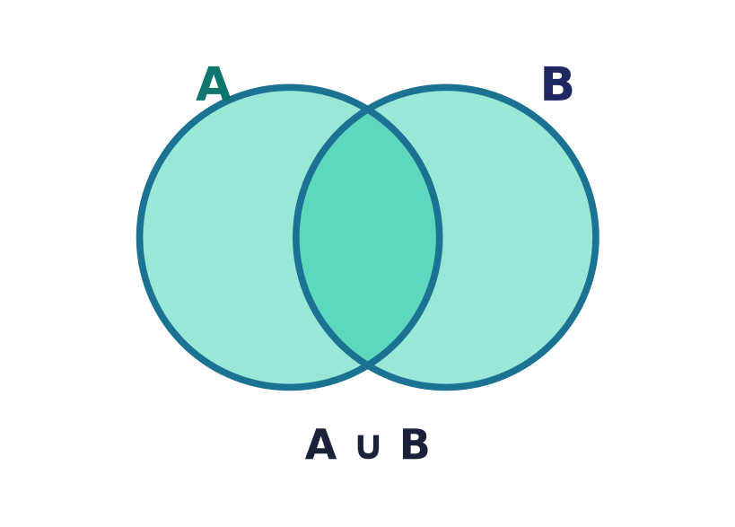
Motivation. To pool two collections into one — the customers who bought product or product , the integers divisible by or by — we want every element that appears in at least one of them.
Definition (union). The union of and is
The “or” is inclusive: an element lying in both sets is included, and — because a set has no duplicates — it is listed only once.
Example 2.1. Let and . Then . The shared elements appear once.
Intersection
Motivation. To find what two collections have in common — the customers who bought both products, the integers divisible by and by (i.e. by ).
Definition (intersection). The intersection of and is
Example 2.2. With the same as above, .
Two order-of-magnitude sanity checks that hold for all :
and if then and (an element already in adds nothing new to the union, and every element of survives the intersection). The containment chain is a one-line element-chase; the equivalences are Exercise S4. Both are used silently all the time.
Difference
Motivation. To remove one collection from another — everyone in who is not also in .
Definition (relative difference). The difference (read “ minus ”) is what remains of after deleting everything that also lies in :
It is not symmetric: in general .
Example 2.3. With , :
keeps the part of outside ; keeps the part of outside . They are different sets — indeed disjoint here.
Complement
Motivation. Often we want “everything except ” — the outcomes of a die that are not a six, the users who did not click. “Everything” must be pinned down, hence the universal set.
Definition (complement). Relative to a fixed universe with , the complement of is everything in not in :
The complement is meaningful only relative to a chosen ; changing changes .
Example 2.4. Take with and . Then
Remark (difference vs. complement). Difference is relative and needs no universe: makes sense for any . Complement is difference from the fixed universe: . Conversely, difference reduces to complement plus intersection: (proved in §2.8). Keeping “relative to what?” in mind avoids many errors.
Common pitfall. has no absolute meaning. If a problem speaks of complements without naming , either is implicit from context (e.g. ) or the problem is ill-posed. Always identify first.
Two identities tie complements to the constants (proved in §2.8):
2.3 Venn diagrams
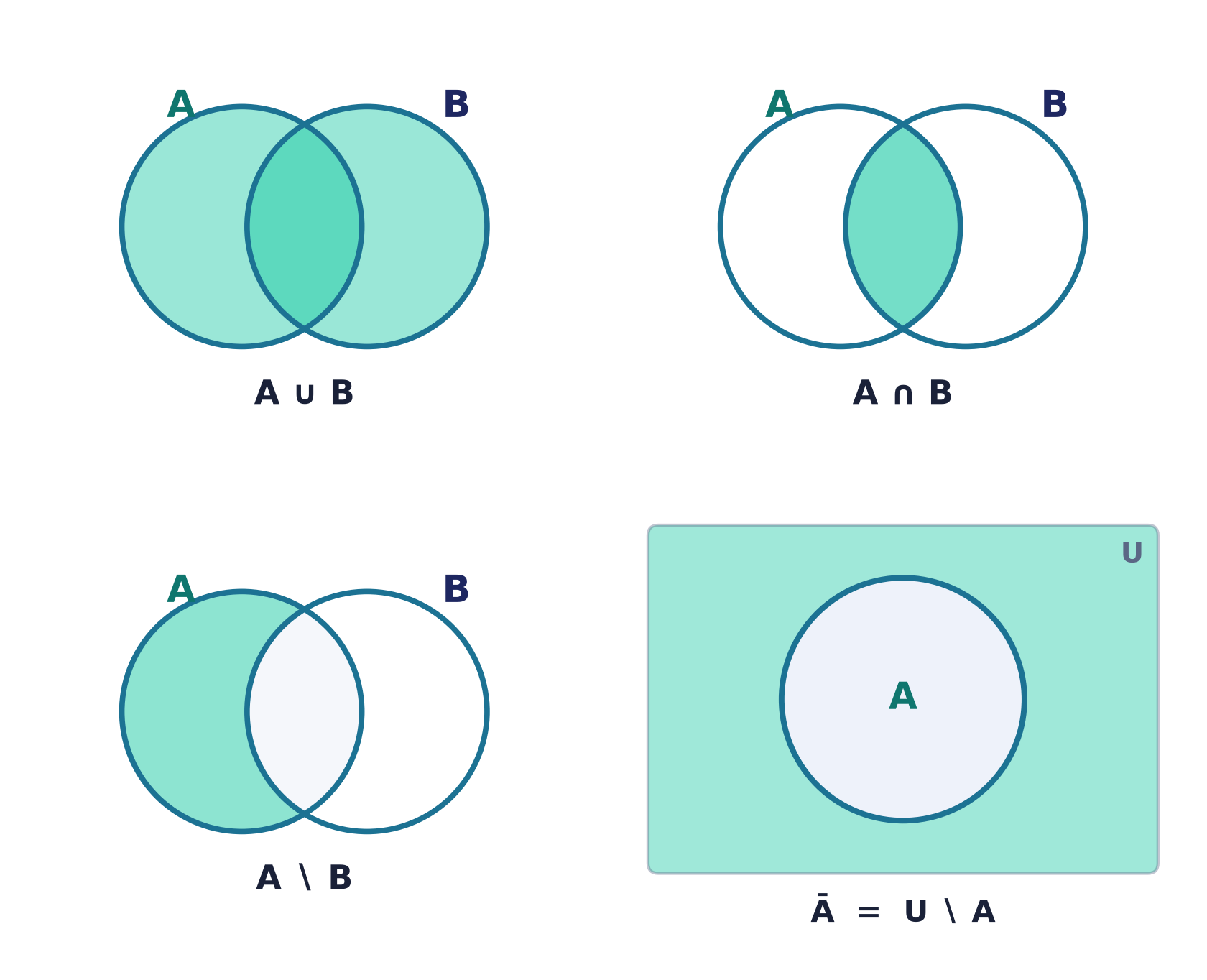
A Venn diagram represents sets as regions — usually circles — inside a rectangle that stands for the universal set . Overlaps show shared elements; shading marks the region an expression denotes. To read an expression off a diagram, shade the part matching its defining predicate: for shade both circles entirely; for shade only the lens-shaped overlap; for shade the crescent of outside ; for shade everything outside circle .
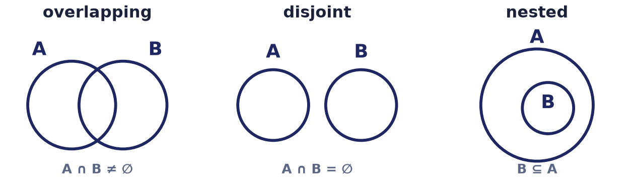
The relative position of two circles encodes the relationship between the sets:
| Configuration | Example | Meaning |
|---|---|---|
| Overlapping circles | , | ; neither contains the other |
| Separate circles | , | (disjoint) |
| One circle inside the other | , |
Remark (a picture is not a proof). With three general circles a Venn diagram has regions (including the outside), one for every combination of “in/out of , , ”, and it faithfully depicts all cases. But for four or more sets three circles cannot show all combinations without distortion, and no finite picture can address arbitrary sets. Diagrams suggest identities and help us understand them; they do not prove them. Proof is the business of §2.8.
2.4 Symmetric difference
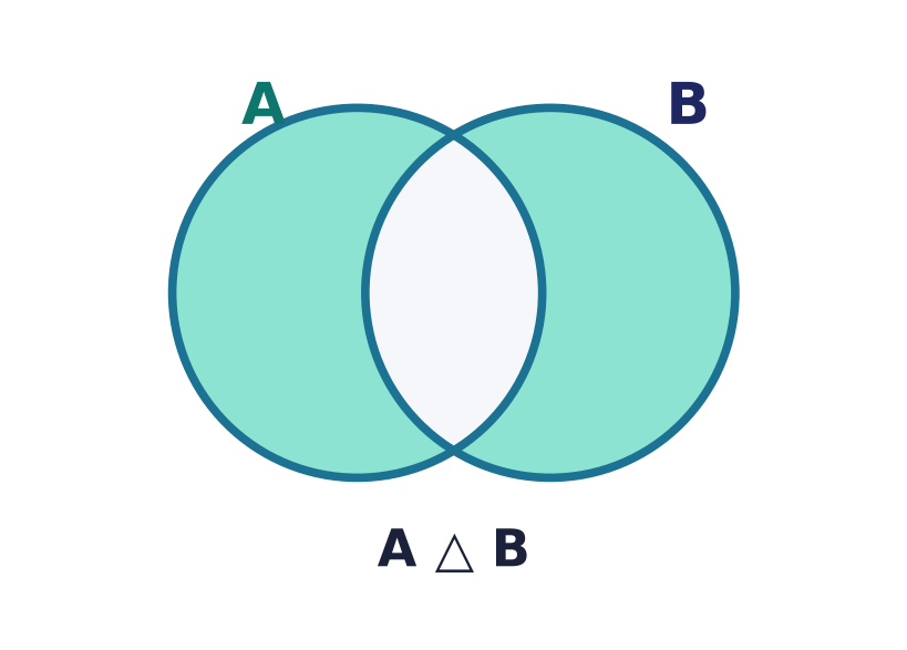
Motivation. The union collects “in or (or both)”; sometimes we want the exclusive version: “in exactly one of , ”. This is the set of elements on which and disagree — the natural notion of “difference between two sets” and, as we will see, the set analogue of the logical XOR and of binary addition.
Definition (symmetric difference). The symmetric difference collects the elements that lie in exactly one of the two sets:
Example 2.5. With , :
These are exactly the elements and disagree on; the agreed-upon drop out.
The definition has a second, equally useful form.
Proposition 2.6.
Proof. We show the two descriptions denote the same set by rewriting one into the other using difference-as-intersection-with-complement (, §2.8) and the laws of §2.7. Starting from the right-hand side and using De Morgan and distributivity:
Distribute the right factor over :
Distribute again inside each bracket:
Now and , and is the identity for , so the expression collapses to
using and commutativity of .
Example 2.7. Rechecking Example 2.5 by the second form: , , so — the same set.
Unlike ordinary difference, symmetric difference is symmetric, and it enjoys a rich algebra developed fully in §2.10:
Because every set is its own inverse (), symmetric difference obeys a cancellation law: (take the symmetric difference of both sides with ).
2.5 Disjoint sets and partitions
Definition (disjoint). Two sets are disjoint if they have no element in common: .
Example 2.8. and are disjoint; their circles do not overlap. and are not disjoint (they share ). Note that and are always disjoint, and both are disjoint from — this three-way split is the key to counting (§2.13).
Definition (pairwise disjoint). A family of sets is pairwise disjoint if whenever .
Disjointness is what makes counting additive: if and are disjoint then with no correction term (the general case is inclusion– exclusion, §2.13).
Definition (partition). A partition of a set is a family of nonempty, pairwise-disjoint subsets whose union is all of . Intuitively, a partition slices into non-overlapping “blocks” that together account for every element exactly once.
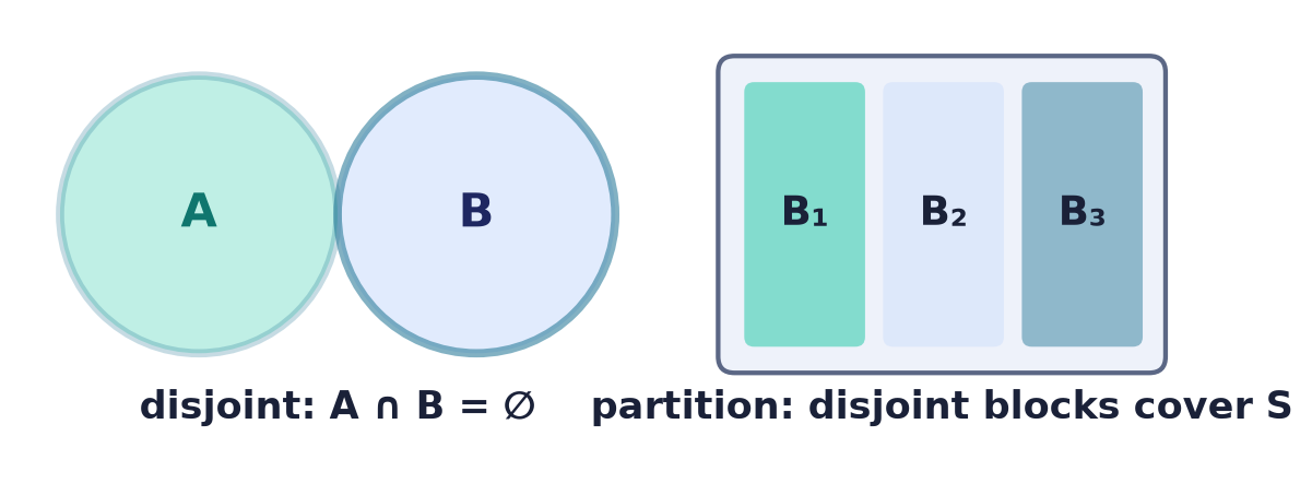
Example 2.9. is a partition of . For any , the pair partitions (assuming both are nonempty). For any two sets, partitions (dropping any empty blocks).
Cross-reference. Partitions are exactly the “quotient” structure produced by an equivalence relation (Lecture 3): each block is an equivalence class. Keep the word in mind; it returns with force there.
2.6 Characteristic functions: the workhorse
Before stating the laws we introduce a device that (i) makes every proof by “membership table” completely rigorous, (ii) reduces set identities to ordinary arithmetic, and (iii) is literally how a computer stores a set. It will pay for itself many times over.
Definition (characteristic function). Fix a universe . The characteristic function (or indicator) of a set is the function given by
A set and its indicator carry exactly the same information, so two sets are equal iff their indicators agree everywhere:
Lemma 2.10 (equality criterion). for all . Likewise for all .
Proof. means for all , i.e. and are both or both — that is, equal — for every . For the subset statement, means , i.e. ; since the values are in this is exactly .
The operations translate into arithmetic on indicators. Here is an arbitrary element of , and all products/sums are ordinary integer arithmetic.
Lemma 2.11 (arithmetic of indicators). For all and all :
Proof. Each is checked by the (at most) four cases of . For intersection: iff and iff iff the product ; otherwise the product is . For complement: iff , so . For union, use the identity (De Morgan) or check directly: if is in neither set both sides are ; if is in exactly one, both sides are (since ); if in both, . Difference and symmetric difference follow from and ; note for the symmetric difference the two terms are disjoint, so the union’s correction term vanishes and , which is when the inputs agree and when they differ — exactly , the XOR.
Finally, indicators count:
Lemma 2.12 (counting via indicators). For finite and ,
Proof. The sum adds for each and for each , so it equals the number of elements of .
Why this matters. Lemma 2.10 turns “prove ” into “prove as functions”, and Lemma 2.11 turns that into an identity of polynomials in the variables — pure algebra, no quantifiers. A membership table (§2.8) is nothing more than evaluating those polynomials at all assignments. And in §2.14 we will see that a characteristic function is a bit-vector, so these lemmas are the specification of the machine’s
AND,OR,NOT,XOR, andpopcount.
2.7 The algebra of sets: the laws
The operations satisfy a fixed collection of identities (laws) holding for all subsets of a universe . They are the axioms/theorems of the algebra of sets. Each law that involves and comes in a pair: swapping and throughout turns one column into the other. This symmetry is the duality principle (§2.9).
| Law | Form 1 (with ) | Form 2 (with ) |
|---|---|---|
| Commutative | ||
| Associative | ||
| Distributive | ||
| Identity | ||
| Domination | ||
| Idempotent | ||
| Complement | ||
| Absorption | ||
| De Morgan | ||
| Double complement | — (self-dual) | |
| Complements of constants |
Two structural remarks worth internalising:
- Associativity lets us drop parentheses and write and unambiguously; more generally and are well-defined (§2.12).
- Distributivity is richer than in arithmetic. In numbers only distributes over (), and does not distribute over . In set algebra both directions hold: over and over . This extra symmetry is exactly what makes the algebra “Boolean”.
Common pitfall (arithmetic intuition misleads). Because resembles and resembles , students expect to fail the way does for numbers. It does not fail: it is a genuine law (Theorem 2.15). Set algebra is not number arithmetic; trust the proofs, not the analogy.
2.8 Proving the laws: two independent methods
There are two standard, fully rigorous ways to prove a set identity , plus the characteristic-function shortcut of §2.6 (which is really Method 1 made algebraic). Mastering both is more important than memorising the laws.
Method 1 — membership table. Every element is classified by which of the sets it belongs to; with sets there are classes, encoded by columns. Build a table with one row per class and columns computing membership in and in (using , , ). If the -column and the -column are identical in every row, then every lies in iff it lies in , so by Lemma 2.10, . (This is exactly evaluating the indicator polynomials of §2.6 at all inputs.)
Method 2 — double inclusion (element-chasing). Prove and separately. For : take an arbitrary , unfold the definitions, and deduce . When every step is an “iff”, the two inclusions are proved simultaneously by a single biconditional chain.
We now prove the core laws, deliberately showing each family by a different method so that both techniques are on display; the flagship distributive law is proved both ways.
Commutativity, associativity, idempotence (biconditional chains)
These three rest directly on the corresponding laws of the logical connectives.
Theorem 2.13 (commutativity). and .
Proof. For every ,
where the middle “iff” is the commutativity of the logical “or”. Since membership in the two sides agrees for every , Lemma 2.10 gives . The case is identical, using commutativity of “and”.
Theorem 2.14 (associativity). and .
Proof. For every ,
the middle step being the associativity of “or”. By Lemma 2.10 the sets are equal. The case uses associativity of “and”.
Theorem (idempotence). and .
Proof. , since is logically equivalent to . Dually .
Remark. Notice the pattern: each set law is the image of a law of propositional logic under the dictionary , , , , . This is not a coincidence; both are Boolean algebras (Lectures 4–5).
Distributivity — proved twice
Theorem 2.15 (distributive law).
Proof 1 (membership table). Three sets give classes. We compute both sides:
| 1 | 1 | 1 | 1 | 1 | 1 | 1 | 1 |
| 1 | 1 | 0 | 1 | 1 | 1 | 0 | 1 |
| 1 | 0 | 1 | 1 | 1 | 0 | 1 | 1 |
| 1 | 0 | 0 | 0 | 0 | 0 | 0 | 0 |
| 0 | 1 | 1 | 1 | 0 | 0 | 0 | 0 |
| 0 | 1 | 0 | 1 | 0 | 0 | 0 | 0 |
| 0 | 0 | 1 | 1 | 0 | 0 | 0 | 0 |
| 0 | 0 | 0 | 0 | 0 | 0 | 0 | 0 |
The two bold columns — membership in and in — agree in all eight rows. By Lemma 2.10 the sets are equal.
Proof 2 (double inclusion). We prove each inclusion by element-chasing.
() Let . Then , and , so or .
- If : then and , so , hence .
- If : then and , so , hence .
In either case . Thus .
() Let . Then or .
- If : then and ; since we have , so .
- If : then and ; since we have , so .
In either case . Thus .
Both inclusions hold, so by the double-inclusion criterion the sets are equal.
Remark (which method when?). Membership tables are mechanical and unambiguous — ideal for checking an identity involving few sets, or when you are unsure it is even true. Double inclusion scales to statements a table cannot reach (arbitrary or infinitely many sets, §2.12) and often reveals why the identity holds. The characteristic-function method (Proof of Proposition 2.6 style, or Lemma 2.11) is the slickest for symbolic manipulation. All three are equally valid; use the one that fits.
The dual law is proved the same way (swap throughout), or derived for free from the duality principle of §2.9.
Absorption — double inclusion and algebraic derivation
Theorem 2.16 (absorption). and .
Proof (double inclusion, first form). () Every satisfies by definition of union, so . () Let . Then , or . In the first case directly; in the second implies . Either way , so . Both inclusions give .
Alternative proof (algebraic, from earlier laws). This shows laws can be derived from laws — the beginning of treating set algebra as a formal calculus:
The second form follows dually.
De Morgan’s laws
De Morgan’s laws describe how complement interacts with union and intersection:
In words: the complement of a union is the intersection of the complements, and the complement of an intersection is the union of the complements. Slogan: “push the bar inward and flip the operation.”
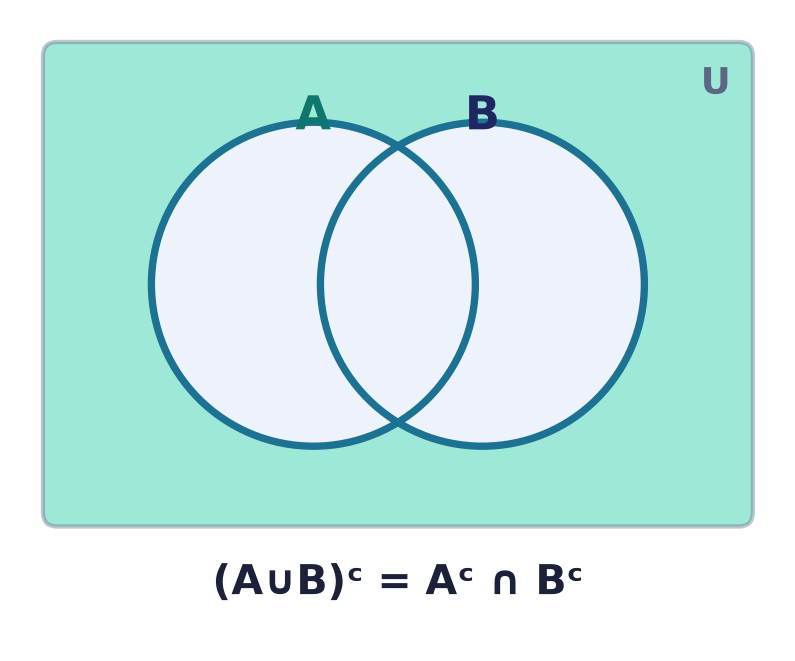
Theorem 2.17 (De Morgan). Both identities above hold for all .
Proof 1 (biconditional chain / double inclusion at once). For every ,
The central step is De Morgan’s law of logic, . Every link is an “iff”, so both inclusions hold and, by Lemma 2.10, .
Proof 2 (membership table). Four classes for the two sets:
| 1 | 1 | 1 | 0 | 0 | 0 | 0 |
| 1 | 0 | 1 | 0 | 0 | 1 | 0 |
| 0 | 1 | 1 | 0 | 1 | 0 | 0 |
| 0 | 0 | 0 | 1 | 1 | 1 | 1 |
The columns and coincide in every row, proving the first law. The second law, , follows by the identical technique, or from the first by replacing with and taking complements (using double complement ), or instantly from duality (§2.9).
Example 2.18. With , , : here , so ; and , , so . Equal, as claimed.
Difference as intersection with complement
We used this identity above; here is its proof, a clean one-line biconditional chain.
Proposition 2.19.
Proof. For all :
This is the bridge that lets any expression in be rewritten purely in , so the laws of §2.7 apply to it. For instance, — a De Morgan-flavoured law for difference (Exercise S3).
2.9 The duality principle
Look again at the table in §2.7: the two columns are mirror images. This is a theorem, not an accident.
Definition (dual). The dual of a set-algebra statement built from (and , , complement) is obtained by interchanging
leaving complements and the sets themselves unchanged. (Under , one also reverses the inclusion, since becomes .)
Duality Principle. If a set identity holds for all subsets of every universe, then so does its dual.
Justification. Take any identity valid for all sets in all universes. Replace every set variable appearing in it by its complement , and then take the complement of both entire sides. Complementing an expression and pushing the bars all the way inward, by repeated De Morgan and double complement, turns every into , every into , every into , every into , and returns each to — precisely the dual transformation. Since the original identity held for all sets (in particular for the complemented ones), the transformed identity also holds universally. That transformed identity is the dual of .
Example 2.20. The distributive law (Theorem 2.15) has dual — applying the swap , gives the other distributive law. Absorption’s two forms are dual; the two De Morgan laws are dual; the two identity laws are mutually dual, as are the two domination laws. Having proved one member of each pair, duality delivers the other for free.
Common pitfall. Duality swaps and only. It does not touch complement bars and does not replace a set by its complement in the final statement. Also, duality is a statement about identities that hold universally; it says nothing about a one-off equation true for some particular sets.
2.10 The algebra of symmetric difference
Symmetric difference deserves its own treatment because it turns into an object with even more structure than the algebra: a ring. The key is Lemma 2.11, which showed — symmetric difference is “addition of indicators modulo ”, i.e. bitwise XOR.
Theorem 2.21 (laws of ). For all :
- Commutative: .
- Associative: .
- Identity: .
- Self-inverse: ; hence .
- distributes over : .
Proof. We work with characteristic functions and Lemma 2.10; write , , , and recall and .
(1) .
(2) , using associativity of integer addition. Since the indicators agree for every , Lemma 2.10 gives equality of the sets.
(3) , so .
(4) , so . For the consequence: if then , i.e. ; as both are this forces , so . Conversely gives .
(5) . Modulo this is , and , , so it equals . (The step holds because multiplication distributes over addition in and reduction mod respects both operations.) Hence the two sets are equal.
CS connection (a Boolean ring). Properties (1)–(5), together with the idempotence and identity , say exactly that is a commutative ring in which every element is its own additive inverse and every element is idempotent under multiplication — a Boolean ring, with “addition” (XOR), “multiplication” (AND), “zero” , and “one” . This is the algebraic heart of digital logic and of Lecture 4–5’s Boolean algebra: XOR is addition mod , AND is multiplication mod . It also explains why solving “set equations” often feels like solving linear systems over the two-element field .
Corollary 2.22 (odd-occurrence rule). For any finite list of sets , an element lies in if and only if belongs to an odd number of the .
Proof. By associativity (Theorem 2.21(2)) the iterated symmetric difference is well-defined, and its indicator at is , which is exactly when an odd number of the summands are , i.e. when is in an odd number of the .
This is the set-theoretic version of “XOR detects odd parity”, the principle behind parity check bits and the classic puzzle of finding the one unpaired element in a list by XOR-ing everything together.
Cardinality of a symmetric difference.
Proof. is a disjoint union, and , (each part of , resp. , outside the overlap). Adding gives . The factor (versus the single subtraction in inclusion–exclusion, §2.13) reflects that the shared elements are excluded from entirely, not merely counted once.
2.11 The Cartesian product
Sets are unordered, but coordinates, records, and strings are ordered. The Cartesian product manufactures order out of unordered sets, and — crucially for Lecture 3 — every relation is a subset of one.
Definition (ordered pair; product). Recall iff and (Lecture 1). The Cartesian product of and is the set of all ordered pairs with first component from and second from :
Example 2.23. , :
nine pairs — one for each choice of first component paired with each choice of second.
Cardinality
Theorem 2.24 (product rule). For finite sets,
Proof. Let and , say with the distinct. Group the pairs of by first coordinate: for each fixed , the set
contains exactly pairs, since distinct ’s give distinct pairs (equality of ordered pairs forces equal second coordinates). Distinct ’s give disjoint (pairs with different first coordinates cannot be equal), and every pair of lies in exactly one . Thus partitions into blocks of size , so by the addition principle (§2.13)
Example 2.25. In Example 2.23, , matching the count.
Algebraic properties, with proofs
Theorem 2.26 (distribution over and ). For all sets :
(The same holds with the product on the right, and with in place of .)
Proof. Elements of these sets are ordered pairs, so we chase a generic pair . For the union:
Distributivity of over rewrites the right side as
Every step is an “iff”, so the two sets have the same elements and are equal. For the intersection, replace the inner by throughout and use idempotence and associativity of (collapsing the duplicated ); the chain becomes .
Theorem 2.27 (behaviour at ; non-commutativity).
- .
- .
- If and are nonempty, then .
Proof. (1) There is no pair whose second (resp. first) component lies in , so the product is empty. (2) If either factor is empty, by (1) the product is empty. Conversely, if both are nonempty, pick , ; then , so the product is nonempty — contrapositive gives the claim. (3) () trivial. () Suppose nonempty and . Take any and any . Then , so has first component in : . As was arbitrary, . Symmetrically for all , so . Hence .
Example 2.28 (non-commutativity). , but — different pairs, so the products differ.
Example 2.29 (distributivity, concrete). , , : , while — the same four pairs.
Common pitfall. The Cartesian product does not distribute over itself, and a union of products need not be a product: is generally not of the form . For example , which is not any Cartesian product (a nonempty product containing and must also contain ). Distribution is of over , not the reverse.
Generalisation: -fold products and powers
For sets we take ordered -tuples:
Example 2.30. Adding to , gives with triples, e.g. , .
When all factors coincide we write the power . In particular is the set of all bit strings of length , with . This set is the same as the set of characteristic functions on an -element universe (§2.6) and the same, up to naming, as for (Lecture 1: ). We exploit this triple identification in §2.14.
Cross-reference (Lecture 3). A binary relation from to is by definition a subset ; an -ary relation is a subset of — the mathematical model of a database table with columns. Everything Lecture 3 does with relations is built on the product defined here, and its cardinality and distributive laws are used there constantly.
2.12 Generalized (indexed) unions and intersections
Union and intersection of two sets extend to an arbitrary family (indexed collection) of sets , where is an index set (possibly infinite).
Definition (generalized union / intersection).
An element qualifies for the union if it lies in at least one member, and for the intersection if it lies in every member. These reduce to the binary operations when , and associativity (Theorem 2.14) guarantees the finite case is unambiguous.
Example 2.31 (finite family). Let for , so , , . Then
For a nested (increasing) family the union is the largest member and the intersection the smallest.
Example 2.32 (infinite families over ). Index by :
Take the first: lies in every interval , while any fails once (choose ), so it is excluded — the intersection is exactly . These examples show generalized operations reaching sets no finite combination produces, which is why element-chasing (Method 2), not tables, is the tool here.
Theorem 2.33 (generalized De Morgan and distributive laws). For any family and any set :
Proof (first De Morgan law). For every ,
the central step being the quantifier duality . By Lemma 2.10 the sets are equal. The other three identities are proved by the same biconditional-chain method, using and the distributive laws of over the quantifiers.
Remark. Membership tables are useless for infinite families (infinitely many “columns”), so Theorem 2.33 can only be proved by element-chasing. This is the concrete reason both proof methods are worth learning: Method 2 is strictly more powerful.
2.13 The inclusion–exclusion principle
Counting the union of sets is the archetype of “correcting for overlap”. Naively adding double-counts the shared elements; inclusion–exclusion is the exact correction. We first isolate the additive foundation.
Addition Principle (rule of sum). If are finite and pairwise disjoint, then .
Proof. By Lemma 2.12, . When the are pairwise disjoint, each lies in at most one of them, so (at most one summand is ). Summing over and swapping the finite sums, .
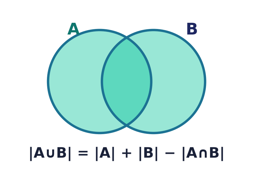
Theorem 2.34 (inclusion–exclusion, two sets). For finite sets ,
Proof (partition into disjoint pieces). The three sets , , are pairwise disjoint and their union is (every element of the union is in only, both, or only). By the addition principle,
Moreover is the disjoint union of and , so , giving ; symmetrically . Substituting into ,
Second proof (characteristic functions). By Lemma 2.11, . Summing over and applying Lemma 2.12 term by term gives at once.
Example 2.35. In a class of students, study French and study German, with studying both. Then study at least one language, and study neither (the neither-count is ).
Theorem 2.36 (inclusion–exclusion, three sets). For finite ,
Proof (reduction to the two-set case). Group and apply Theorem 2.34:
By the distributive law (Theorem 2.15), ; apply Theorem 2.34 to this union:
Now by commutativity and idempotence. Substitute (Theorem 2.34) and into :
which rearranges to the stated formula.
The pattern — add singles, subtract pairwise overlaps, add back the triple overlap — continues.
Remark (general inclusion–exclusion). For finite sets,
i.e. add all singletons, subtract all pairs, add all triples, and so on with alternating signs. It follows by expanding (the union’s complement is the intersection of the complements) and summing over : the product expands into a signed sum of over subsets , exactly the alternating formula.
2.14 Applications
2.14.1 Bit-vector set operations
Everything in §2.6 becomes a data structure. Fix a universe of size with a chosen ordering . Represent a subset by its bit vector whose -th bit is : bit is iff . This is the characteristic function written as a binary word — the identification of §2.11 made physical.
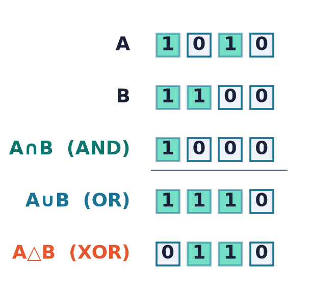
Under this representation, Lemma 2.11 says the set operations are exactly the bitwise machine instructions:
| Set operation | Bitwise op on | Indicator identity |
|---|---|---|
OR |
||
AND |
||
NOT |
||
AND with NOT : a & ~b |
||
XOR |
||
| ? | test bit : (a >> i) & 1 |
|
popcount (population count) |
Worked example. Let and index element to bit . For and (our running sets):
Then
matching Examples 2.1–2.5 exactly. De Morgan’s law appears at the hardware level as
NOT(a OR b) == (NOT a) AND (NOT b).
CS connection. For a set fits in one machine word, so union, intersection, membership, and complement each cost a single CPU instruction, and costs one
POPCNT. For larger universes one uses words (), giving time — the constant-factor speedup behindstd::bitset(C++),BitSet(Java),roaring bitmapsin databases, and Python’s arbitrary-widthintused as a bit set. Sieve of Eratosthenes, graph reachability by bitset propagation, and DNA -mer sets all lean on this. The duality principle even tells the compiler that an expression and its dual compile to the same-length instruction sequence withAND/ORswapped.
2.14.2 Inclusion–exclusion counting
Inclusion–exclusion turns “count things avoiding several forbidden properties” into arithmetic. The template: let be the set of objects having property ; count the union by Theorem 2.34/2.36; subtract from the total to count objects with none of the properties.
Example 2.37 (divisibility). How many integers in are divisible by , , or ? Let be the multiples of respectively. The count of multiples of in is , and a number is divisible by both and (coprime) iff divisible by :
By Theorem 2.36,
So integers are divisible by at least one of , and are divisible by none (i.e. coprime to ).
Example 2.38 (survey). Among people, use product , use , use ; use and , use and , use and , and use all three. Then
so use at least one product and use none.
Common pitfall. The pairwise data must be the sizes of the intersections (“use both and ”), not “use exactly and and nothing else”. If a problem gives exactly-counts (region-by-region), do not plug them into Theorem 2.36; instead fill the Venn regions directly and add. Mixing the two conventions is the most common inclusion–exclusion error.
2.14.3 SQL set operations
A relational database table, under set semantics, is a set of rows (tuples), so the algebra of this chapter is literally the algebra of query results. Standard SQL provides three set operators, applied to two union-compatible queries (same number of columns, compatible types) — the SQL echo of “you can only combine sets drawn from the same universe”:
| Set operation | SQL | Notes |
|---|---|---|
A UNION B |
duplicates removed (true set union) | |
A INTERSECT B |
||
A EXCEPT B (Oracle: A MINUS B) |
||
(A EXCEPT B) UNION (B EXCEPT A) |
no dedicated keyword | |
SELECT * FROM U EXCEPT SELECT * FROM A |
complement needs an explicit universe table U |
For instance, students taking at least one of two languages, and those taking both:
SELECT id FROM french_students
UNION
SELECT id FROM german_students;      -- ∪ : at least one

SELECT id FROM french_students
INTERSECT
SELECT id FROM german_students;      -- ∩ : both

SELECT id FROM french_students
EXCEPT
SELECT id FROM german_students;      -- ∖ : French but not German
Common pitfall (bag vs. set semantics). Plain
UNIONremoves duplicate rows — matching the mathematical union — butUNION ALLkeeps them, implementing multiset (bag) union, which does not obey idempotence ( when has rows). The distinct-preserving operators (UNION,INTERSECT,EXCEPT) obey all the laws of §2.7; theALLvariants generally do not. Because deduplication costs a sort or hash, engines use bag semantics by default in many contexts — know which one your query is in.
Cross-reference. SQL’s
WHEREclause combines conditions withAND,OR,NOT, which by the logic–set dictionary correspond to , , complement on the selected row-sets — soWHERE p AND qselects the intersection of the rows satisfyingpand those satisfyingq. The full theory of tables as -ary relations is Lecture 3.
Historical note
The algebra of sets is a nineteenth-century creation. George Boole (1815–1864), in The Mathematical Analysis of Logic (1847) and An Investigation of the Laws of Thought (1854), recast logic as algebra — his “elective symbols” combine essentially as and do here, and the laws of §2.7 are, in modern dress, Boole’s laws (Lectures 4–5 return to “Boolean algebra” by name). Augustus De Morgan (1806–1871), Boole’s correspondent and a founder of symbolic logic, gave the complement–union–intersection laws that bear his name. John Venn (1834–1923) introduced his diagrams in an 1880 paper on the diagrammatic representation of propositions. The set-theoretic universe of objects to which these operations apply was supplied by Georg Cantor (1845–1918), whose work in the 1870s–1880s founded set theory as an autonomous subject. The inclusion–exclusion principle grew from work of Abraham de Moivre and was cast as a general counting principle by J. J. Sylvester in the nineteenth century. Finally, the observation that is a ring (§2.10) is part of the bridge between Boolean algebras and ring theory made precise by Marshall Stone in the 1930s (Stone’s representation theorem). Thus a single small algebra sits at the meeting point of logic, set theory, combinatorics, and abstract algebra — and, a century later, of digital hardware.
Chapter summary
- The basic operations are union (in either), intersection (in both), difference (in not ), complement (in not ), and symmetric difference (in exactly one). Each is defined by a logical predicate on membership; (Prop. 2.19) reduces difference to the others.
- Venn diagrams picture sets as regions in ; they illustrate but do not prove identities beyond a handful of sets.
- Sets are disjoint when ; a partition slices a set into nonempty pairwise-disjoint blocks. Disjointness makes counting additive.
- The characteristic function identifies a set with a function and turns operations into arithmetic ( product, , complement , XOR); . Set equality indicator equality (Lemma 2.10).
- The algebra of sets obeys commutative, associative, distributive (both ways!), identity, domination, idempotent, complement, absorption, De Morgan, and double-complement laws, arranged in dual pairs. Each is a shadow of a law of propositional logic.
- A set identity is proved by a membership table (finitely many sets) or by double inclusion / biconditional chains (any sets, including infinite families) — and often most slickly by characteristic functions. The distributive and De Morgan laws were proved by more than one method.
- The duality principle (, ) gives the dual of any universally valid identity for free.
- Symmetric difference is commutative, associative, has identity and is self-inverse (); distributes over it, making a Boolean ring. An element is in iff it lies in an odd number of the sets.
- The Cartesian product is the set of ordered pairs, with (Thm 2.24); it distributes over (Thm 2.26), is non-commutative for distinct nonempty factors (Thm 2.27), and generalises to -tuples and powers — including bit strings . It is the foundation of relations (Lecture 3).
- Generalized unions/intersections range over arbitrary indexed families and obey generalized De Morgan and distributive laws (Thm 2.33), provable only by element-chasing.
- The inclusion–exclusion principle counts unions by correcting for overlap: and the three-set formula (Thms 2.34, 2.36), with an alternating-sign generalisation to sets.
- Applications: bit vectors realise sets as machine words with operations;
inclusion–exclusion solves “at least one / none” counting; SQL’s
UNION,INTERSECT,EXCEPTare on tables (with a bag-vs-set caveat).
Exercises
Warm-up
W1. For and , compute , , , , and .
W2. With and , find . Then change to and find again. Explain in one sentence why the answer changed.
W3. For , , compute both as and as , and check the two agree. Verify .
W4. Let with element stored in bit . Write the -bit
vectors of and , then compute ,
, and by bitwise OR, AND, XOR, and translate each
back to a set.
W5. List all elements of . How many elements does have, and why does this equal for ?
W6. In a group of people, like tea, like coffee, and like both. How many like at least one drink? How many like neither?
W7. State the dual of each: (a) ; (b) ; (c) .
Standard
S1. Prove the absorption law by double inclusion.
S2. Prove the distributive law by a membership table (all rows).
S3. Using and the laws of §2.7, prove and .
S4. Prove that the following are equivalent for all sets : (i) ; (ii) ; (iii) . (Hint: prove (i)(ii)(iii)(i) by element-chasing.)
S5. Prove by chasing a generic ordered pair.
S6. Of students, took calculus, took linear algebra, and took discrete math; took calculus and linear algebra, took calculus and discrete math, took linear algebra and discrete math, and took all three. How many took at least one of the three courses? How many took none?
S7. Prove the cardinality identity , and use it to find when , , .
S8. Compute, for the family (): and . Justify each with a one-line element argument.
S9. Given two tables A(id) and B(id), write SQL statements returning the ids
in (a) , (b) , (c) , (d) . State one
reason A UNION ALL B can differ from A UNION B.
Challenge
C1. Prove that symmetric difference is associative, , using characteristic functions, and deduce that iff lies in an odd number of . Then list for , , .
C2. (a) Prove . (b) Give sets showing need not be a Cartesian product.
C3. Prove the two-set inclusion–exclusion principle using characteristic functions (sum over ), then extend the same idea to re-derive the three-set formula by expanding .
C4. How many integers in are divisible by none of ? (Use four-set inclusion–exclusion; the general alternating formula in §2.13 helps.)
C5. Prove that satisfies the ring axioms with “zero” and “one” : additive associativity/commutativity, additive identity and inverses, multiplicative associativity/identity, and distributivity of over . Which extra property makes it a Boolean ring? (Connect to Lectures 4–5.)
C6. In a three-set Venn diagram you are told: , , , , exactly elements lie in and (whether or not in ), exactly lie in , exactly lie in , and . Find the number of elements in exactly one of the three sets, and the number in none.
Selected answers & hints
W1. ; ; ; ; .
W2. (for ), then (for ). Complement is measured against , so enlarging enlarges .
W4. , ; ; ; .
W5. The eight strings ; . Each bit string is a characteristic function on the -element universe, and characteristic functions correspond bijectively to subsets, so this equals .
W6. like at least one; like neither.
W7. (a) ; (b) ; (c) .
S2. Table columns ; the fifth and eighth columns both read down the eight rows (order from to ) — hint: is whenever , and when it is iff .
S4. (i)(ii): if then (both parts lie in ) and always, so . (ii)(iii): by absorption. (iii)(i): if then every satisfies , hence ; so .
S6. took at least one; took none.
S7. is the disjoint union of and , of sizes and ; sum is . Numerically .
S8. : for all , and any fails once . : the sets are nested decreasing, so the union is the largest, .
C1. With (mod ), ; the value is iff is odd, i.e. an odd number of memberships. For the given sets, element counts are , so the odd ones are : .
C3. Summing over and using gives . Expanding and using etc. yields ; sum over .
C4. Total ; let be multiples of . Singles: . Pairs (multiples of ): . Triples (of ): . Quadruple (of ): . Then . Divisible by none: .
C6. “Exactly in and ” here means (the standard reading: in both, regardless of ); similarly , . Then , so are in none. For “exactly one”: elements in only (subtract the two pairwise overlaps involving , add back the triple counted out twice); only ; only . Total in exactly one .
Further reading
- K. H. Rosen, Discrete Mathematics and Its Applications. Chapter 2 (Sets, set operations, set identities) and the treatment of inclusion–exclusion; Rosen’s membership-table and “show each is a subset” proofs parallel §2.8, and his bit-string representation of sets matches §2.14.1.
- S. S. Epp, Discrete Mathematics with Applications. The chapter on set theory develops the element-method (double inclusion) proofs in careful detail — excellent companion reading for §2.8 and §2.12.
- For the algebraic viewpoint (Boolean algebras and Boolean rings, §2.10) and the duality principle, see the Boolean-algebra chapters of the same texts, previewing Lectures 4–5 of this course.