Lecture 6. Propositional logic
6.0 Overview and motivation
In Lecture 4 and Lecture 5 we studied Boolean algebra: an algebraic structure with operations , , and complement on the two-element set , together with a body of laws (commutativity, distributivity, De Morgan, and the rest). We manipulated expressions the way we manipulate ordinary algebra — by rewriting, factoring, and simplifying.
Propositional logic is the same machinery seen from a different angle — the angle of meaning and truth rather than algebraic manipulation. Instead of bits and gates we now speak of propositions (declarative sentences), the connectives that glue them together, and the central question: when is a compound sentence true? The two subjects are, quite literally, two dialects of one theory. Where Lecture 4 wrote we now write ; where it wrote we now write . This is not a loose analogy — it is an isomorphism, and §6.9 makes it precise.
Why build a formal language for something as ordinary as “and”, “or”, and “if”? Three reasons, each a theme of the whole course:
- Precision. Natural language is ambiguous (“or” can be inclusive or exclusive; “if” is often mistaken for “if and only if”). A formal language forces every sentence to have exactly one structure and exactly one truth value per interpretation.
- Mechanization. Once meaning is reduced to a finite table lookup, a machine can check whether an argument is valid, whether a circuit meets its specification, or whether a configuration of constraints can be satisfied. This is the birthplace of automated reasoning, SAT solvers, and hardware/software verification.
- Foundation for proof. Every proof you will write in Lecture 7 and beyond — direct proof, contraposition, contradiction, cases — is a disciplined way of establishing exactly the semantic relationships defined here. You cannot say what a proof proves until you can say what its statements mean.
We treat propositional logic as a formal system in three layers, and this lecture is organized around them:
- Syntax (§6.5) — what counts as a legal formula: well-formed formulas, connectives, parenthesization, precedence, parse trees. Pure grammar, no truth involved.
- Semantics (§6.6) — how a formula acquires a truth value once we fix the truth values of its atoms: interpretations, the recursive definition of truth, truth tables.
- Meta-theory (§6.7–§6.11) — classifying formulas (tautology, contradiction, contingency), testing satisfiability (SAT), deciding when two formulas mean the same thing (), reducing formulas to normal forms (CNF, DNF), and deciding when a sentence follows from others ().
Remark (where we stop). This lecture is about truth, decided ultimately by inspecting a truth table. How to derive consequences by rules of inference (modus ponens, natural deduction) and how to organize those rules into proof techniques belongs to Lecture 7. The distinction — semantics () versus proof theory () — is fundamental and is drawn explicitly in §6.12. Keep it in mind throughout: here, nothing is ever “derived”; everything is computed or checked.
6.1 Statements and propositions
Definition (proposition). A statement (or proposition) is a declarative sentence that is either true or false, but not both and not neither.
The two possible values form the tiny truth-value set , written or . Whether we currently know which value a sentence has is irrelevant; what matters is that it has exactly one. “There are infinitely many twin primes” is a perfectly good proposition even though, at the time of writing, no one knows whether it is true.
Consider the sentences a logic course traditionally opens with:
- “The Dnipro flows into the Black Sea.” — a statement; it happens to be true.
- “The Dnipro flows into the Sea of Azov.” — a statement; it happens to be false.
- “What’s the date today?” — not a statement. It is a question; it cannot be assigned or .
Sentences that are not propositions include:
- questions — “What time is it?”;
- commands / imperatives — “Close the door.”;
- exclamations — “How cold it is!”;
- paradoxical self-referential sentences — “This sentence is false.” If it were true it would be false, and if false, true; it can be assigned neither value consistently, so it lies outside the realm of propositions altogether. (This is the Liar paradox, and the care needed to exclude such sentences is one reason a formal syntax matters.)
Definition (open sentence). A sentence containing a free variable whose truth value depends on the value substituted for that variable is an open sentence (a propositional function or predicate).
A subtler case than the ones above is “ is divisible by 5.” This has no fixed truth value on its own: it depends on . It becomes a genuine proposition only after is given a concrete value — for it is true, for it is false. Propositional logic treats only closed sentences with definite truth values; open sentences, together with the quantifiers “for all” () and “there exists” () needed to close them, are the subject of predicate (first-order) logic, which the course takes up later.
Example 6.1 (classification). Classify each sentence. (a) “ is a prime number.” (b) “Please pass the salt.” (c) “ for the integer .” (d) “Is it raining?” (e) “.”
Solution. (a) proposition, true. (b) not a proposition (imperative). (c) proposition, true — the variable is bound by the phrase “for the integer ”, which quantifies it, so the sentence as a whole makes a definite (true) claim. (d) not a proposition (question). (e) open sentence — true when , false otherwise; a proposition only once is fixed.
Common pitfall. Do not confuse “we don’t know its truth value” with “it has no truth value.” The Goldbach conjecture is a proposition (exactly one of true/false), even though its status is open. By contrast “” genuinely has no truth value until is supplied — it is a different kind of object, an open sentence.
6.2 Atomic and compound propositions
Definition (atom). An atom (atomic proposition) is a simple declarative sentence that contains no logical connective and cannot be decomposed into smaller propositions — “a simple narrative sentence.” Atoms are the indivisible building blocks of the language. We denote them by propositional variables: (or ).
Definition (compound proposition). A compound (or molecular) proposition is one built from atoms using logical connectives.
The defining feature of the language is captured by one principle:
Principle of truth-functionality. The truth value of a compound proposition is determined completely by the truth values of its atoms together with the meanings of its connectives — and by nothing else.
Truth-functionality is a genuine restriction, and it is what makes the whole theory computable. It says the connective “and” contributes only a rule for combining truth values; it is blind to what the atoms say, whether they are related in meaning, whether one causes the other, or whether they are even about the same topic. The compound “ and Kyiv is a city” is true for exactly the same reason as “grass is green and snow is white”: both conjuncts are true. English connectives sometimes smuggle in extra meaning (temporal order in “she opened the door and left”); propositional logic deliberately discards all of that.
Example 6.2. “Peter was late” is an atom, say . “Peter was late and Peter was speeding” is compound: , where is the atom “Peter was speeding.” The whole sentence carries no truth value of its own beyond what , , and supply.
6.3 Logical connectives
Propositional logic uses five standard connectives. Negation is unary (applies to one formula); the other four are binary (combine two).
| Connective | Symbol | Reads as | Natural-language cues |
|---|---|---|---|
| Negation | “not ” | not; it is not the case that; fails to | |
| Conjunction | “ and ” | and; but; both … and; yet; although | |
| Disjunction | “ or ” | or; either … or (inclusive) | |
| Implication | “if then ” | if …, then …; only if; implies; is sufficient for | |
| Biconditional | “ if and only if ” | iff; exactly when; is necessary and sufficient for |
Each connective is defined by how it computes a truth value; those definitions are the rows of the base truth table in §6.6. Four points of natural-language nuance deserve emphasis now.
(1) “But” is . Logically, “it is raining but the sun is shining” is just the conjunction . English uses “but” to signal contrast or surprise; truth-functionally there is no such thing, and is true precisely when both parts are.
(2) Disjunction is inclusive. is true when at least one of holds, including when both hold. English “or” is sometimes exclusive (“soup or salad, not both”); that meaning is a different connective, exclusive-or , expressible as
When a menu says “soup or salad” it means ; when a scholarship says “open to students who study mathematics or computer science” it means (a double major still qualifies). Which one is intended is a matter of translation, not of logic.
(3) Implication is truth-functional and needs no causal link. is false in exactly one case: antecedent true and consequent false. In every other case it is true. In particular, when the antecedent is false, is vacuously true, regardless of — “if the moon is made of cheese, then ” is a true implication. Here is the antecedent (hypothesis) and the consequent (conclusion). Implication captures the pattern “ is guaranteed whenever ”, not “ causes ”.
(4) The four English faces of . All of the following translate to : “if , then ”; “ only if ”; “ is sufficient for ”; “ is necessary for ”; “ whenever ”; “ follows from .” The two easy-to-miss ones are “only if” and “necessary”: “ only if ” does not say — it says that can hold only in circumstances where also holds, i.e. .
Related to are three formulas built from the same atoms; distinguishing them is a constant source of error:
- converse: ;
- inverse: ;
- contrapositive: .
Common pitfall (affirming/denying traps). A conditional is not equivalent to its converse or its inverse. “If it rains, the ground is wet” () does not entail “if the ground is wet, it rained” (converse — the sprinkler could be on) nor “if it does not rain, the ground is not wet” (inverse). It is equivalent to its contrapositive “if the ground is not wet, it did not rain” — a fact we prove in §6.9 and use constantly in Lecture 7.
Remark (other connectives). Two further binary connectives matter in computer science: NAND and NOR . §6.10 shows every connective can be expressed with ; remarkably, NAND alone (or NOR alone) also suffices, which is why entire chips are built from one gate type.
6.4 Formalization: from natural language to formulas
Formalization (translation, symbolization) is the act of replacing atoms by variables and connective-words by symbols. It is the first practical skill of the subject and the bridge between messy language and computable logic.
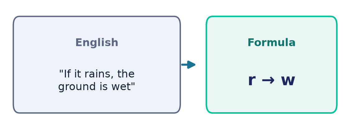
The method:
- Identify the atomic propositions and assign each a variable. Choose atoms to be positive where possible (let = “the door is open”, not “the door is closed”), so that negations show up explicitly.
- Locate the connective words (“and”, “or”, “if…then”, “not”, “unless”, “only if”, …).
- Determine the grouping (scope) — this is the step that requires judgment — and insert parentheses accordingly.
Example 6.3 (the “Peter” sentence). “Because Peter was late, he was speeding, and therefore he is not a good driver.” Atoms: = “Peter was late”, = “Peter was speeding”, = “Peter is a good driver”. The sentence asserts: if (Peter’s being late led to ) then not . Formalized:
Translation is not mechanical: cue words guide it, but scope and grouping require reading the sentence’s intent. The placement of “not” is especially treacherous.
Example 6.4 (scope of negation). “Not both and ” — at least one fails. “Both not and not ” — both fail. These are genuinely different formulas: the first is true when , the second is not. (By De Morgan, , so the first equals “ or ” — note the or.)
Example 6.5 (“unless”). “You will pass unless you cheat.” Read “ unless ” as “ if not ”, i.e. , equivalently . With = “you pass”, = “you cheat”:
Example 6.6 (“neither…nor” and “only if”). “Neither nor ” . “ only if ” (not !). “ if ” . “ if and only if ” .
Example 6.7 (a compound argument to formula). “If the program compiles and the tests pass, then we deploy; we did not deploy; the tests passed. So the program did not compile.” Atoms = “compiles”, = “tests pass”, = “we deploy”. Premises: . Conclusion: . (We check whether this argument is valid in §6.11.)
Common pitfall (the “and”/“or” reversal after “not”). Everyday speech says “you can’t have cake and ice cream” to mean you can have at most one — logically , which is . The English keeps “and”, but the correct paraphrase uses “or”. Always translate the meaning, then let De Morgan reconcile it with the words.
6.5 Syntax: well-formed formulas
Syntax is grammar with truth deliberately set aside. Before we can ask what a formula means, we must fix exactly which strings of symbols are formulas. This matters for the same reason a compiler has a grammar: only well-formed input can be assigned a meaning, and the meaning must be unambiguous.
Definition (well-formed formula). The well-formed formulas (WFFs) of propositional logic over a set of propositional variables are defined by recursion:
- (base) Every propositional variable is a WFF (an atom).
- (negation) If is a WFF, then is a WFF.
- (binary) If and are WFFs, then , , , and are WFFs.
- (closure) Nothing else is a WFF.
Clause 4 is essential: it says the WFFs are the smallest set closed under 1–3. This is what licenses the two most important tools of the subject — proof by structural induction and definition by structural recursion.
Thus is well-formed, while , , and are not.
Remark (fully parenthesized vs. readable). The definition above puts parentheses around every application, which makes the theory clean but the formulas ugly. In practice we drop the outermost parentheses and the parentheses around negation, and we use precedence and associativity conventions to reinsert the rest.
Precedence and associativity. From tightest binding (evaluated first) to loosest:
Binary connectives associate to the right, so abbreviates . Under these rules,
Common pitfall (association of ). Right-association is a convention for abbreviation, not a logical law: and are not equivalent. Their truth tables differ:
F F F F T F F T T T F T F F T F T T T T T F F T T T F T T T T T F F F T T T T T The columns disagree in rows 1 and 3. When in doubt, write the parentheses.
Parse trees and the main connective
Every WFF corresponds to a unique parse tree (syntax tree): leaves are atoms, internal nodes are connectives, and each connective’s children are the trees of its immediate subformulas. The connective at the root — the one applied last — is the main connective. Identifying the main connective is the key step in reading and evaluating a formula, because it tells you the outermost structure.
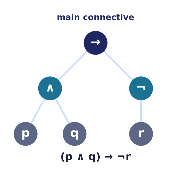
Example 6.8. The parse tree of :
           ∧            ← main connective
         /   \
        →     ¬
       / \     \
      p   q     r
The main connective is ; its left subtree is and its right subtree is . Contrast:
- In the main connective is the second (left subtree , right subtree ).
- In the main connective is , applied to the whole conjunction.
- In the main connective is (because binds tighter): left subtree , right subtree .
Unique readability
The convenience of precedence rules rests on a theorem that is easy to take for granted and surprisingly delicate to prove: a well-formed formula can be parsed in exactly one way. Without this, “the main connective” and “the truth table” would not even be well defined.
Theorem 6.1 (Unique Readability). Every WFF is of exactly one of the following forms, and in each case its parts are uniquely determined:
- an atom ; or
- for a unique WFF ; or
- for a unique binary connective and unique WFFs .
Proof. For a string over our alphabet, let be the number of “” minus the number of “” occurring in . We first establish two lemmas.
Lemma A. Every WFF satisfies . We argue by structural induction on . If is an atom it contains no parentheses, so . If then by the induction hypothesis. If then . This proves Lemma A.
Lemma B. Every proper, nonempty prefix of a WFF satisfies . (A prefix is proper if it is not all of .) Again by structural induction on .
- Base. An atom has length , hence no proper nonempty prefix; the claim holds vacuously.
- Negation, . A proper nonempty prefix is one of: “” (then ); “” (then ); “” where is a nonempty prefix of . If is a proper prefix of , then by the induction hypothesis; if (the whole thing), then by Lemma A.
- Binary, . Enumerate the proper nonempty prefixes: “” (); “” with a proper nonempty prefix of (); “” (); “” (); “” with a proper nonempty prefix of (); “” (). Every case gives .
This proves Lemma B.
Consequence. No proper nonempty prefix of a WFF is itself a WFF, since a WFF has (Lemma A) but such a prefix has (Lemma B).
Now the theorem. The first symbol of a WFF determines its form: a WFF beginning with a propositional letter is that atom (atoms have length and no other clause produces a string starting with a letter); a WFF beginning with “” followed by “” is a negation; a WFF beginning with “” followed by anything else is a binary formula. So the three forms are mutually exclusive. For uniqueness within the binary case, suppose as strings. Deleting the leading “” gives . The substrings and both begin at the first position, so one is a prefix of the other; if they had different lengths, the shorter would be a proper nonempty prefix of the longer WFF — impossible by the Consequence. Hence , so the connective symbols align, giving , and therefore . The negation case is immediate (the inner formula is the unique substring between “” and the matching final “”). ∎
Remark. Theorem 6.1 is the propositional analogue of a parser proving its grammar is unambiguous. The proof technique — a numeric invariant () plus structural induction — is exactly how one reasons about balanced brackets in compilers and about balanced-parenthesis languages in formal language theory. It is why the abbreviation conventions (dropping parentheses, using precedence) are safe: each abbreviation names one and only one fully parenthesized WFF.
6.6 Semantics: interpretations and truth tables
Syntax says which strings are formulas; semantics says what they mean. Meaning here is entirely a matter of truth values.
Definition (interpretation). An interpretation (truth valuation, assignment) is a function
assigning a truth value to every atom.
Because the connectives are truth-functional, an interpretation of the atoms forces the truth value of every formula built from them. The next theorem makes “forces” precise and rigorous — it is the semantic counterpart of Unique Readability.
Theorem 6.2 (the valuation extends uniquely). For every interpretation of the atoms there is a unique function from all WFFs to satisfying:
- for every atom ;
- if , and otherwise;
- iff and ;
- iff or ;
- iff and , and otherwise;
- iff .
Proof. Existence. Define by structural recursion on , using clauses 1–6. By Theorem 6.1 every WFF matches exactly one of the forms atom / negation / binary, so exactly one clause applies at each step and the recursion is well defined; its value is computed from the strictly smaller immediate subformulas, so the recursion terminates. The resulting satisfies 1–6 by construction.
Uniqueness. Suppose and both satisfy 1–6. We show for all WFFs by structural induction. If is an atom, by clause 1. If , then by the induction hypothesis , and clause 2 computes and from that common value, so they agree. The binary cases are identical, using the induction hypothesis on both immediate subformulas and the relevant clause 3–6. Hence . ∎
We henceforth write for both the assignment and its extension , and introduce the satisfaction symbol.
Definition (satisfaction, model). For an interpretation and formula , write
read “ satisfies ” or “ is a model of .” We write when .
A formula with distinct atoms has exactly interpretations (each atom independently or ) — these are precisely the rows of its truth table.
The base connective table. Theorem 6.2’s clauses, tabulated with atoms :
| F | F | T | F | F | T | T |
| F | T | T | F | T | T | F |
| T | F | F | F | T | F | F |
| T | T | F | T | T | T | T |
Read the rows as definitions: conjunction is true only when both conjuncts are true; disjunction is false only when both disjuncts are false; implication is false only in the row ; the biconditional is true exactly when and agree.
Remark (row ordering). We list rows with before , reading each row as a binary number with counting upward (). Any fixed order works; consistency is what matters, and we keep this one throughout the lecture.
Building a truth table. To evaluate a compound formula, introduce one column per subformula, ordered by the parse tree (atoms first, main connective last). Each column is computed from earlier columns via the base table.
Example 6.9. Truth table for (main connective ):
F F T T T F T T F F T F F T F T T T F F The bold final column is the value of the whole formula under each of the interpretations. It is true only when .
Example 6.10 (three atoms, eight rows). Truth table for :
F F F F T T F F T F F F F T F F T T F T T F F F T F F F T T T F T F F F T T F T T T T T T T F T False exactly when and not both hold.
6.7 Classifying formulas: tautology, contradiction, contingency
Looking only at the final column of a formula’s truth table, every formula falls into exactly one of three classes.
Definitions.
- A tautology is a formula true under every interpretation (final column all ). Also called logically valid; we write . Example: (law of excluded middle).
- A contradiction is a formula false under every interpretation (final column all ). Example: .
- A contingency is a formula true under some interpretations and false under others. Example: .
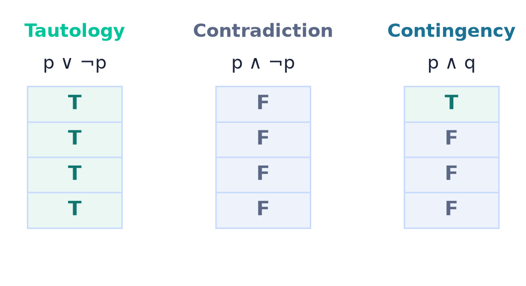
These classes partition the set of all formulas: every formula is exactly one of the three. They are linked by negation.
Theorem 6.3 (tautology–contradiction duality). A formula is a tautology if and only if is a contradiction; and is a contradiction if and only if is a tautology.
Proof. By clause 2 of Theorem 6.2, for every interpretation we have iff . Now: is a tautology for all for all is a contradiction. The second statement follows by applying the first to and using double negation (, Theorem 6.7). ∎
Example 6.11 (verify a tautology). Show (a conditional is equivalent to its contrapositive).
F F T T T F T T T T T F F F T T T T T T The final column is all , so the formula is a tautology. (The two inner columns are equal — foreshadowing in §6.9.)
6.8 Satisfiability and the SAT problem
Definition (satisfiability). A formula is satisfiable if at least one interpretation makes it true — i.e. its final column contains at least one . A formula with no satisfying interpretation is unsatisfiable.
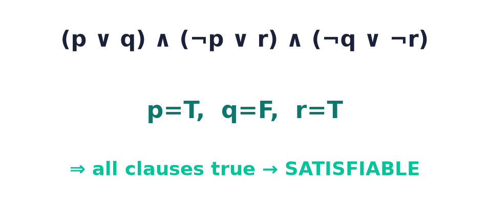
Thus unsatisfiable = contradiction, while tautologies and contingencies are satisfiable. The following little theorem ties satisfiability to the classification of §6.7 and to validity, and is the theoretical basis of refutation-style reasoning.
Theorem 6.4 (satisfiability/validity duality). A formula is a tautology if and only if is unsatisfiable.
Proof. is a tautology for all no has no has is unsatisfiable. ∎
Definition (joint satisfiability). A set of formulas is jointly (simultaneously) satisfiable if some single interpretation makes all of them true at once — equivalently, if the conjunction is satisfiable.
Example 6.12. Is a tautology, contradiction, or contingency, and is it satisfiable?
whole F F F T F F T T T T T F T T T T T T F F Mixed final column contingency, hence satisfiable (e.g. by ). It is true exactly when exactly one of holds — it is the exclusive-or .
The SAT problem
The Boolean satisfiability problem (SAT) is the decision problem: given a propositional formula, is it satisfiable? A truth table always answers it — build the table, scan for a — but the table has rows for atoms, so the naive method becomes hopeless well before (already rows).
SAT is a landmark of theoretical computer science:
- Cook–Levin Theorem (1971). SAT was the first problem proved NP-complete (Stephen Cook; Leonid Levin independently). Informally, NP-complete problems are the hardest problems whose candidate solutions can be checked quickly; SAT is a “universal” such problem, in that every problem in NP reduces to it. Whether SAT admits a worst-case polynomial-time algorithm is the famous open P vs. NP question. No efficient worst-case algorithm is known, and most researchers conjecture none exists.
- In practice, SAT is astonishingly tractable. Modern SAT solvers based on the DPLL procedure (Davis–Putnam–Logemann–Loveland) and its modern extension CDCL (conflict-driven clause learning) routinely settle formulas with millions of variables. They exploit structure — unit propagation, learning from conflicts, clever branching — rather than enumerating all rows.
Why CS cares. SAT (and its close cousins) is the engine behind:
- Hardware verification / equivalence checking: to prove two circuits compute the same function, assert they differ on some input and let a SAT solver try to satisfy that assertion; unsatisfiable means the circuits are equivalent (this is exactly Theorem 6.4 at industrial scale — recall Lectures 4–5, where circuits are Boolean formulas).
- Model checking of hardware and software (does this system ever reach a bad state?).
- Planning, scheduling, and configuration (encode constraints as clauses; a model is a valid plan/schedule).
- Program analysis and symbolic execution (path conditions are formulas; feasibility is satisfiability).
Remark (validity is co-SAT). By Theorem 6.4, testing whether is a tautology is the same as testing whether is unsatisfiable. So tautology-checking (a validity question) and SAT (a satisfiability question) are two sides of one coin, and a single SAT solver handles both.
6.9 Logical equivalence
Definition (logical equivalence). Two formulas and are logically equivalent, written , if they have the same truth value under every interpretation — identical final columns in the truth table.
Note the level distinction, which trips up many beginners:
Common pitfall ( vs. ). The symbol is a connective: is itself a formula, which may be true under some interpretations and false under others. The symbol is a meta-level assertion about two formulas — a statement in our mathematical English, not a symbol inside the logic. The next theorem is the precise bridge between them.
Theorem 6.5 (equivalence via the biconditional). if and only if is a tautology. Moreover, is an equivalence relation on formulas: it is reflexive, symmetric, and transitive.
Proof. By clause 6 of Theorem 6.2, for each interpretation , iff . Therefore is a tautology iff for every , which is exactly the definition of .
For the equivalence-relation claim, work directly from the definition. Reflexive: for all , so . Symmetric: if for all , then for all , so . Transitive: if and for all , then for all , so . ∎
The next theorem is what lets us reason algebraically — replacing a subformula by an equivalent one anywhere inside a larger formula, exactly as we substitute equals in ordinary algebra.
Theorem 6.6 (substitution / replacement). Let be a formula containing as a subformula, and let be the result of replacing that occurrence of by . If , then .
Proof. Fix any interpretation ; since we have . We show by structural induction on , where is with the marked occurrence of replaced by .
- If the marked occurrence is all of , then and , and .
- Otherwise the occurrence lies strictly inside , so is not an atom. If , the occurrence is inside ; by the induction hypothesis , and clause 2 gives . If for a binary , the occurrence lies in or in ; the induction hypothesis gives and (the untouched side is unchanged), and the clause for then gives .
Since was arbitrary, . ∎
The equivalence laws
The following laws are the working toolkit. Each is a claim that two formulas are equivalent, and each is verifiable by a truth table (and provable from the others by algebra via Theorem 6.6).
| Law | Form |
|---|---|
| Double negation | |
| Idempotence | , |
| Commutativity | , |
| Associativity | , |
| Distributivity | , |
| De Morgan | , |
| Identity | , |
| Domination | , |
| Complement | , |
| Absorption | , |
| Implication | |
| Contrapositive | |
| Biconditional |
Remark (this is Lecture 4 again). These are exactly the Boolean-algebra laws of Lecture 4, with in place of , in place of , and in place of . The map carrying to the two-element Boolean algebra is an isomorphism: propositional logic is the two-element Boolean algebra, read semantically. Everything you proved algebraically there holds here, and vice versa.
Now we discharge the task of actually proving the load-bearing laws. Truth tables are the direct method; each is a finite check of “same final columns.”
Theorem 6.7 (double negation). .
Proof.
| F | T | F |
| T | F | T |
The columns and are identical. ∎
Theorem 6.8 (De Morgan’s laws). and .
Proof. First law:
| F | F | F | T | T | T | T |
| F | T | F | T | T | F | T |
| T | F | F | T | F | T | T |
| T | T | T | F | F | F | F |
Columns and agree . Second law:
| F | F | F | T | T | T | T |
| F | T | T | F | T | F | F |
| T | F | T | F | F | T | F |
| T | T | T | F | F | F | F |
Columns and agree . ∎
Theorem 6.9 (distributivity). and .
Proof. First law (the second is dual; its table is checked the same way):
| F | F | F | F | F | F | F | F |
| F | F | T | T | F | F | F | F |
| F | T | F | T | F | F | F | F |
| F | T | T | T | F | F | F | F |
| T | F | F | F | F | F | F | F |
| T | F | T | T | T | F | T | T |
| T | T | F | T | T | T | F | T |
| T | T | T | T | T | T | T | T |
The two boldfaced-in-comparison columns are both . ∎
Theorem 6.10 (implication as disjunction). .
Proof.
| F | F | T | T | T |
| F | T | T | T | T |
| T | F | F | F | F |
| T | T | T | F | T |
Columns and agree . ∎
This law is the most useful of all: it lets us eliminate entirely and rewrite any formula using only — the first step of the normal-form algorithm in §6.10.
Theorem 6.11 (contrapositive). .
Proof.
| F | F | T | T | T | T |
| F | T | T | F | T | T |
| T | F | F | T | F | F |
| T | T | T | F | F | T |
Columns and agree . ∎
Theorem 6.12 (biconditional). .
Proof.
| F | F | T | T | T | T | F | T | T |
| F | T | F | T | F | F | F | F | F |
| T | F | F | F | T | F | F | F | F |
| T | T | T | T | T | T | T | F | T |
The columns , , and are all . ∎
Reasoning algebraically
By Theorem 6.6 we may chain equivalences, substituting inside larger formulas, without ever drawing a truth table. This is often far faster.
Example 6.13 (simplify ).
So “not ( implies )” means exactly “ holds but fails” — matching the single -row () of the implication table.
Example 6.14 (simplify ). Using Theorem 6.12 then De Morgan and distribution,
That last formula is the exclusive-or of Example 6.12 — so , confirming that “not equivalent” means “exactly one holds”.
Example 6.15 (a chain to ). Show is a tautology by algebra.
(Steps: implication; De Morgan; commutativity/associativity; complement; domination.) A formula provably equal to is a tautology.
6.10 Normal forms: CNF and DNF
Normal forms are standardized shapes into which every formula can be rewritten. They matter because algorithms (SAT solvers, circuit synthesizers, Lecture 4–5 minimization) expect their input in a fixed shape.
Definitions.
- A literal is an atom or the negation of an atom: or .
- A clause is a disjunction of literals, e.g. .
- A term (implicant) is a conjunction of literals, e.g. .
- A formula is in conjunctive normal form (CNF) if it is a conjunction of clauses: — an “AND of ORs”.
- A formula is in disjunctive normal form (DNF) if it is a disjunction of terms: — an “OR of ANDs”.
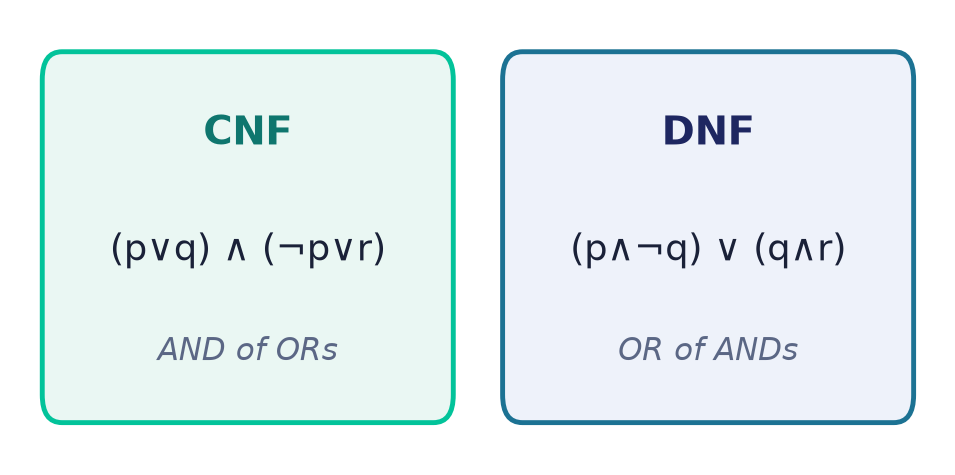
Remark (which is which). Mnemonic: CNF = Conjunction on the outside; DNF = Disjunction on the outside. CNF is the input format demanded by SAT solvers. DNF makes satisfiability trivial to read off (a DNF is satisfiable iff some term contains no complementary pair ) but can be exponentially large.
Theorem 6.13 (existence of normal forms). Every propositional formula is logically equivalent to a formula in DNF and to a formula in CNF.
Proof. We give a constructive proof from the truth table of ; let its atoms be .
DNF. If is a contradiction, then , which is (a degenerate) DNF. Otherwise, for each interpretation with (each true row), form the minterm
By construction is true under and false under every other interpretation (any other interpretation disagrees with on some , making that literal false, hence the whole conjunction false). Let . For any interpretation : if then the disjunct is true, so is true; if then every disjunct (with , ) is false at , so is false. Hence has the same truth value as everywhere: , and is in DNF.
CNF. Dually, if is a tautology then (a degenerate CNF). Otherwise, for each interpretation with (each false row), form the maxterm
i.e. the negation of the pattern of . Then is false under and true under every other interpretation. Let . A symmetric argument shows , and is in CNF. (Alternatively: apply the DNF construction to , then negate and push negations in with De Morgan — De Morgan turns the DNF of into a CNF of .) ∎
Corollary 6.14 (functional completeness). The set of connectives is functionally complete: every truth function of variables is computed by some formula using only .
Proof. A truth function is a final column, i.e. the truth table of some formula; Theorem 6.13 produces an equivalent DNF (or CNF), which uses only . ∎
Remark. Because and (De Morgan), even and are complete; and a further reduction shows NAND alone and NOR alone are each complete (the Sheffer stroke, proved complete in print by Sheffer in 1913 and anticipated by Peirce around 1880). This is exactly why digital hardware (Lectures 4–5) can be built entirely from NAND gates.
Obtaining normal forms by rewriting
The truth-table method of Theorem 6.13 is canonical but produces large formulas. In practice one rewrites, in three stages:
- Eliminate and using and .
- Push negations inward to the atoms using De Morgan and double negation, reaching negation normal form (NNF) — where appears only directly on atoms.
- Distribute: for CNF, distribute over ; for DNF, distribute over .
Example 6.16 (to CNF by rewriting). Convert .
The result is in CNF. Meanwhile is already in DNF (a disjunction of the one-literal term and the term ).
Example 6.17 (to DNF by rewriting). Convert . Distributing over :
a DNF with four terms. (This one-formula example already shows how distribution can multiply out: two clauses of size 2 became four terms.)
Example 6.18 (NNF via De Morgan).
Negations now sit only on atoms (NNF), and the result is in DNF.
Example 6.19 (canonical forms of ). From its truth table (; false only at ):
- Canonical DNF (minterms for the three true rows ): .
- Canonical CNF (maxterm for the one false row ): .
The CNF collapses to the single clause — precisely Theorem 6.10. This illustrates that canonical forms are correct but not minimal; minimization (Karnaugh maps, Quine–McCluskey) is the Lecture 4–5 topic.
6.11 Logical consequence and validity of arguments
We can now make precise what it means for a conclusion to follow from premises — the central notion of correct reasoning.
Definition (logical consequence / entailment). Given premises and a conclusion , the premises entail , written
if every interpretation that makes all the premises true also makes true. Equivalently: there is no interpretation (no counterexample) satisfying all premises yet falsifying . Read as “semantically entails” or “yields.”
Definition (valid argument). An argument with premises and conclusion is valid exactly when ; otherwise it is invalid, and any interpretation making all premises true and the conclusion false is a counterexample.
The following theorem reduces every entailment question to a tautology (hence, via Theorem 6.4, to a satisfiability) question — the reason a single truth-table procedure decides validity.
Theorem 6.15 (semantic deduction theorem). if and only if the formula is a tautology.
Proof. Write . For any interpretation , iff satisfies all the premises.
() Assume . Take any . If , then (implication with false antecedent). If , then satisfies all premises, so by entailment , whence . Either way is true under ; as was arbitrary, is a tautology.
() Assume is a tautology. Let satisfy all premises, so . Since and the antecedent is true, the consequent . Thus every model of all premises is a model of , i.e. . ∎
Theorem 6.16 (entailment via unsatisfiability — refutation). if and only if is jointly unsatisfiable.
Proof. fails iff some satisfies all but not , i.e. satisfies all and — i.e. iff is jointly satisfiable. Negating both sides gives the claim. ∎
Remark (why refutation matters). Theorem 6.16 is how automated reasoners actually test entailment: to check , throw in with the premises and ask a SAT solver whether the result is unsatisfiable. “Unsatisfiable” is the proof. This is the semantic seed of the proof by contradiction technique you will meet in Lecture 7.
Common pitfall (validity ≠ true premises). Validity is about form — the transmission of truth — not about whether the premises are actually true. A valid argument can have false premises and a false conclusion; validity only guarantees that if the premises are true, the conclusion must be. Conversely, an argument can have a true conclusion yet be invalid (the conclusion just happens to hold, not because the premises force it).
Worked validity checks
The truth-table test for : build one table; scan only the rows where all premises are true; the argument is valid iff the conclusion is true in every such row.
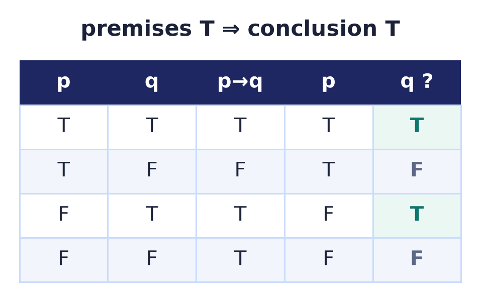
Example 6.20 (modus ponens — valid). “If it rains, the ground is wet. It rains. Therefore the ground is wet.” Let = “it rains”, = “the ground is wet”. Premises ; conclusion .
F F T F F F T T F T T F F T F T T T T T Both premises are true only in the last row, where the conclusion is also true. No counterexample valid. (Reached purely by inspecting truth values; the name “modus ponens” and its use as a derivation rule belong to Lecture 7.)
Example 6.21 (affirming the consequent — invalid). “If it rains, the ground is wet. The ground is wet. Therefore it rains.” Premises ; conclusion . The row makes both premises true (, ) yet the conclusion . That is a counterexample, so — invalid, despite its surface resemblance to Example 6.20.
Example 6.22 (hypothetical syllogism — valid). .
F F F T T T F F T T T T F T F T F T F T T T T T T F F F T F T F T F T T T T F T F F T T T T T T Both premises are true in rows 1, 2, 4, 8; in each of those the conclusion is true. No counterexample valid.
Example 6.23 (modus tollens — valid). .
F F T T T F T T F T T F F T F T T T F F Both premises true only in row 1, where . Valid. Contrast denying the antecedent : rows make both premises true, but at the conclusion — a counterexample, so that pattern is invalid.
Example 6.24 (the deploy argument, Example 6.7). Premises ; conclusion . Suppose all premises hold: gives ; gives . If were , then , and the first premise would force , contradicting . So , i.e. . Every model of the premises satisfies the conclusion — valid. (This informal case analysis is exactly what a truth table verifies row by row, and what Theorem 6.15 packages as the tautology .)
The same truth-table method thus does triple duty in this lecture: it classifies a single formula (§6.7), it tests equivalence of two formulas by comparing final columns (§6.9), and it tests validity of an argument by scanning for a counterexample row (§6.11).
6.12 Semantics versus proof theory (a bridge to Lecture 7)
Everything above is semantic: truth values, interpretations, truth tables, and the entailment symbol . We answered “does follow from ?” by checking all interpretations.
Lecture 7 takes the complementary, proof-theoretic (syntactic) route. It fixes a small stock of rules of inference — modus ponens (“from and , infer ”), modus tollens, disjunctive syllogism, and so on — and defines a derivation as a finite chain of formulas, each an axiom, a premise, or the result of applying a rule to earlier lines. Here nothing is “true” or “false”; formulas are manipulated by rules, mechanically, like moves in a game.
| Semantics (this lecture) | Proof theory (Lecture 7) | |
|---|---|---|
| Central relation | (entailment) | (derivability) |
| Basic object | truth value, interpretation | inference rule, derivation |
| Method | truth tables / model search | rule application / proof construction |
| Question answered | is it true in all models? | can it be derived? |
The two views are connected by two deep meta-theorems, which the course states (and Lecture 7 uses) but which are proved in a dedicated logic course:
- Soundness: if then (the rules never derive a falsehood from truths — proofs are trustworthy).
- Completeness (Gödel, 1929/30, for first-order; the propositional case is Post, 1921): if then (every genuine entailment can be derived — the rules are enough).
Together, for propositional logic, and coincide: derivability and entailment are the same relation, approached from two directions. That is why the proof techniques of Lecture 7 are correct (soundness) and sufficient (completeness) for exactly the semantic facts established here.
Historical note
The algebraic treatment of logic began with George Boole, whose The Mathematical Analysis of Logic (1847) and An Investigation of the Laws of Thought (1854) reduced reasoning to calculation on the symbols and — the origin of “Boolean algebra” (Lectures 4–5). Augustus De Morgan, Boole’s contemporary, gave the duality laws that bear his name. Gottlob Frege’s Begriffsschrift (1879) introduced a rigorous formal language with a precise notion of well-formed formula, launching modern mathematical logic and the syntax/semantics distinction of §6.5–§6.6. The truth table as a systematic device is usually credited to Ludwig Wittgenstein (Tractatus, 1921) and Emil Post (1921) independently, with earlier anticipations by Charles S. Peirce; Post also proved the first functional-completeness results. Jan Łukasiewicz devised parenthesis-free “Polish notation,” reminding us that unique readability (Theorem 6.1) can be achieved by grammar alone. In computer science, Claude Shannon’s 1937 master’s thesis identified propositional logic with switching circuits — the direct ancestor of Lectures 4–5 — and Stephen Cook (1971), with Leonid Levin independently, proved SAT NP-complete, placing propositional satisfiability at the very center of computational complexity.
Chapter summary
- A proposition/statement is a declarative sentence with a definite truth value in . Questions, commands, exclamations, paradoxical sentences, and open sentences like “ is divisible by ” are not propositions.
- Atoms are indivisible simple sentences (propositional variables). Compound propositions are built from atoms with and are truth-functional: their value depends only on the atoms’ values and the connectives.
- Key connective facts: is inclusive; is false only when (vacuously true when ); is equivalent to its contrapositive but not its converse or inverse.
- Syntax defines well-formed formulas by recursion; precedence and parentheses fix a unique parse tree with a main connective. Unique Readability (Theorem 6.1) guarantees exactly one parse.
- Semantics: an interpretation assigns values to atoms and extends uniquely to all formulas (Theorem 6.2); means is true under . A formula with atoms has interpretations — the rows of its truth table.
- Every formula is a tautology (always ; ), a contradiction (always ), or a contingency (mixed). It is satisfiable iff some interpretation makes it true. is a tautology iff is unsatisfiable (Theorem 6.4).
- SAT — deciding satisfiability — is the first NP-complete problem (Cook–Levin); truth tables solve it in steps, while real SAT solvers (DPLL/CDCL) scale to millions of variables and power verification, planning, and analysis tools.
- Logical equivalence (equal columns; equivalently a tautology, Theorem 6.5) is an equivalence relation and supports substitution (Theorem 6.6). The laws — double negation, De Morgan, distributivity, , contrapositive, biconditional — are proved by truth tables (Theorems 6.7–6.12) and are the semantic twins of the Boolean-algebra laws of Lecture 4.
- Every formula has an equivalent DNF and CNF (Theorem 6.13), obtained canonically from the truth table or by rewriting (eliminate ; push inward to NNF; distribute). Consequently is functionally complete (Corollary 6.14).
- Entailment holds when every model of is a model of ; an argument is valid iff there is no counterexample row, iff (premises conclusion) is a tautology (Theorem 6.15), iff is unsatisfiable (Theorem 6.16).
- This lecture is about meaning and truth (); deriving consequences with rules of inference () and proof techniques is Lecture 7, tied back by soundness and completeness.
Exercises
Warm-up
- Decide which are propositions; for those that are, give the truth value if known. (a) “ is prime.” (b) “Solve the equation .” (c) “.” (d) “Every even integer is a sum of two primes.” (e) “This exercise is hard!”
- Write the negation, converse, inverse, and contrapositive of “If a number is divisible by , then it is divisible by .” Which of the four is guaranteed to have the same truth value as the original?
- Insert full parentheses according to the precedence rules and identify the main connective: (a) ; (b) ; (c) .
- Build the truth table of and classify it (tautology / contradiction / contingency).
- Translate into symbols with stated atoms: (a) “I will go running unless it snows.” (b) “You may enter only if you have a ticket.” (c) “Neither the printer nor the scanner works.”
Standard
- Build the truth table of and classify it. On which interpretations is it false?
- Prove by truth table that (the second distributive law).
- Using equivalence laws only (cite each step, no truth table), simplify: (a) ; (b) ; (c) .
- Show that (constructive-dilemma pattern). Use a truth table or a short case argument, and identify the rows where all premises hold.
- Determine, with a truth table, whether the argument is valid: “If the cache is warm, the request is fast. The request is not fast. Therefore the cache is not warm.”
- Find a DNF and a CNF for (exclusive-or) and for . (You may read them off truth tables.)
- Convert to CNF by rewriting (show stages): .
- Is ? Justify by finding all models of the premises and checking the conclusion.
- Show that (the “exportation” law) by any method, and explain why this does not contradict the non-equivalence of and from §6.5.
Challenge
- (Unique readability in action.) Explain why the string needs the precedence convention to be read, and exhibit the two different fully parenthesized WFFs it could abbreviate. Show by truth table that they are not equivalent, so the convention (not mere taste) is doing real work.
- (Functional completeness.) Show that is functionally complete by expressing , , and using only and . (Hint: start from .)
- (NAND.) Let . Express , , and using only , thereby proving NAND is functionally complete by itself.
- (Refutation.) Use Theorem 6.16 to test : write the set , argue it is unsatisfiable, and explain how “unsatisfiable” certifies the entailment.
- (Compactness of the method, and its cost.) A formula has distinct atoms. (a) How many rows does its truth table have? (b) Explain why deciding satisfiability by truth table is impractical for , giving the approximate row count. (c) State in one sentence what a SAT solver does differently.
- (Modeling.) Three suspects are questioned. says “ did it.” says “I didn’t do it.” says “I didn’t do it.” Exactly one suspect is guilty and exactly one statement is true. Introduce atoms for guilt, encode the constraints as a propositional formula, and determine the guilty party.
Selected answers & hints
1. (a) proposition, true. (b) not a proposition (imperative). (c) open sentence — a proposition only once is fixed. (d) proposition (this is Goldbach’s conjecture — its truth value is unknown, but it has one). (e) not a proposition (exclamation, and subjective).
2. Original (“divisible by ” “divisible by ”). Negation: . Converse: . Inverse: . Contrapositive: . Only the contrapositive is guaranteed equivalent (Theorem 6.11); the original is true here, its contrapositive true, but its converse (“divisible by divisible by ”) is false ( is a counterexample).
3. (a) , main connective . (b) , main connective . (c) , main connective .
4. : the column is — a contingency, false only at (there , so ; when the implication is vacuously true, and when the consequent is true).
5. (a) , i.e. , with =“I run”, =“it snows”. (b) (“only if” antecedent is enter), =“enter”, =“have ticket”. (c) .
6. False exactly when is true but is false — i.e. the row (there , ). So it is a contingency, false only at .
8. (a) (De Morgan then double negation). (b) — a tautology. (c) .
9. Valid. In any row where is true, at least one of holds; together with / that forces . No row has all three premises true and false.
10. Valid — this is modus tollens (); cf. Example 6.23.
11. : DNF ; CNF . : DNF ; CNF .
12. — a single clause, already CNF.
14. Both sides equal (rewrite each with the implication law and associate). No contradiction with §6.5: there we compared with — different left-hand sides — whereas here the left side is the conjunction , not the implication .
15. It could abbreviate or . Truth tables differ (e.g. : the first is , the second is ). The convention selects the first reading; without it the string would be ambiguous.
16. Using only : (since ); ; and a contradiction (as is a tautology). Having reconstructed , Corollary 6.14 finishes completeness.
17. ; ; . (Verify each by a - or -row table.)
18. From and we need ; from and we need ; but demands — no interpretation satisfies all four, so the set is unsatisfiable, which by Theorem 6.16 certifies (this is two chained modus-ponens steps, a.k.a. the transitivity of ).
19. (a) . (b) rows — beyond any feasible enumeration. (c) A SAT solver searches assignments intelligently (unit propagation, conflict-driven clause learning), pruning the space instead of listing all rows.
20. Let mean “// is guilty.” Statements: , , . Constraints: exactly one of is true (guilt) and exactly one of is true (truth). Now and are negations of each other, so exactly one of them is true no matter what; since only one statement in total may be true, must be false. Then gives , so is guilty, and exactly-one-guilty forces innocent. Check: with we get — exactly one true statement (). The model is unique. C did it.
Further reading
- K. H. Rosen, Discrete Mathematics and Its Applications — Chapter 1, “The Foundations: Logic and Proofs,” especially §1.1 (propositional logic), §1.2 (applications), §1.3 (propositional equivalences). The standard CS-oriented treatment, with many translation and circuit examples.
- S. S. Epp, Discrete Mathematics with Applications — Chapter 2, “The Logic of Compound Statements” (statements, connectives, truth tables, logical equivalence, conditionals, valid arguments). Especially clear on natural-language translation and the converse/inverse/contrapositive distinctions.
- H. B. Enderton, A Mathematical Introduction to Logic — Chapter 1, for the rigorous syntax/semantics development (unique readability, the valuation theorem, functional completeness) at the level of §6.5–§6.6 and §6.10.
- M. Huth & M. Ryan, Logic in Computer Science: Modelling and Reasoning about Systems — for CNF, SAT/DPLL, and the verification applications sketched in §6.8.
- Cross-references within this course: Lectures 4–5 (Boolean algebra and logic circuits — the same algebra, read algebraically) and Lecture 7 (rules of inference and proof techniques — the syntactic counterpart, , to this lecture’s ).