Lecture 10. Graph theory — basics
Overview
A graph is a mathematical model of a collection of objects together with the pairwise connections between them. The objects are drawn as dots and the connections as lines, which makes graphs one of the most visual — and most widely applicable — structures in discrete mathematics. Computer networks, road maps, web-page link structures, molecule diagrams, task-dependency charts, and social networks are all naturally described by graphs.
This lecture builds the vocabulary of graph theory from the ground up. We define graphs and directed graphs, fix the core terminology (adjacency, incidence, degree, loops, parallel edges, the Handshaking Lemma), catalogue the special families we reuse constantly (null, complete, complete bipartite), and give two matrix representations (adjacency and incidence). We then formalise movement through a graph — walks, trails, paths, circuits, cycles — touch on connectivity, and finish with three structural questions: when are two graphs the same (isomorphism), when can a graph be drawn without crossings (planarity and Kuratowski’s theorem), and how few colours suffice to colour it (chromatic number and index).
What separates this chapter from a bare glossary is proof. Almost every claim below — the Handshaking Lemma, the edge counts of and , the fact that matrix powers count walks, Euler’s formula, the non-planarity of and — is stated as a theorem and proved. Learning to read and reproduce these proofs is the real content of the course; the definitions are only the alphabet.
Concrete algorithms for graphs — breadth- and depth-first search, shortest paths, minimum spanning trees, and greedy colouring — are the subject of Lecture 11, while special families such as trees, together with Euler and Hamilton tours, are studied in Lecture 12. Here we build only the language and its theory. Directed graphs reappear as the transition diagrams of finite automata in Lecture 14.
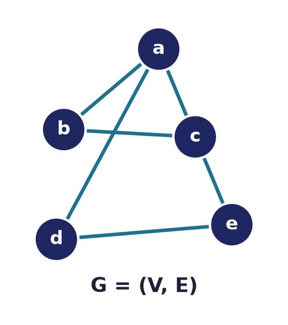
Throughout the lecture we reuse one running example:
10.1 A historical note: the bridges of Königsberg
Graph theory has a precise birthday. In 1736 Leonhard Euler settled a puzzle about the Prussian city of Königsberg (today Kaliningrad), which straddled the river Pregel around two islands connected to the banks and to each other by seven bridges. The townspeople asked: can one take a stroll that crosses every bridge exactly once and returns home?
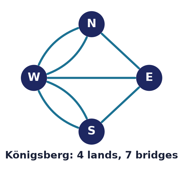
Euler’s insight was to throw away all geometric detail. The four landmasses become four vertices; each bridge becomes an edge joining the two masses it connects. The question is now purely combinatorial: does this graph admit a closed walk using every edge exactly once (what we now call an Eulerian circuit)? Euler observed that whenever such a walk enters a landmass by one bridge it must leave by another, so every vertex must have even degree. In Königsberg the four vertices had degrees — all odd. Since
the degrees obey the Handshaking Lemma of §10.4 (their sum is twice the number of bridges), yet four of them are odd, and no walk of the desired kind can exist.
Two things make this the founding example of the subject. First, it abstracts a concrete situation into vertices and edges — the modelling move we repeat constantly. Second, its solution turns on a degree condition, exactly the kind of counting argument this chapter develops. The systematic theory of Eulerian circuits and their construction belongs to Lecture 12; here Königsberg motivates why degrees and their parities are worth studying so carefully.
10.2 Graphs and directed graphs
A graph consists of a non-empty set of vertices (also called nodes or points) and a set of edges (also lines), where each edge joins an unordered pair of vertices. We write for the number of vertices (the order of the graph) and for the number of edges (the size). An edge joining vertices and is written or ; because the pair is unordered, and denote the same edge.
Commentary: the whole of the graph lives in the pair ; the drawing is a convenience for humans, and — as isomorphism (§10.10) will make precise — the same graph has infinitely many drawings. Two vertices are joined or they are not; how long or curved the line is carries no information (until we add weights in §10.7).
A simple graph has no loops and no parallel edges (both defined in §10.3); unless stated otherwise, “graph” means “simple graph”. Formally, in a simple graph is a set of -element subsets of . A graph that does allow parallel edges (so that is a multiset) is a multigraph.
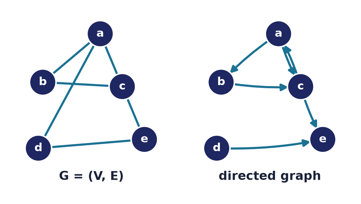
A directed graph (or digraph) replaces edges by arcs (directed edges): each arc is an ordered pair , drawn as an arrow from the tail to the head . Now and are different arcs — direction matters. Digraphs model one-way relationships: one-way streets, web hyperlinks (page links to page ), prerequisite chains, task dependencies, or the transitions of a finite automaton (Lecture 14).
Example. The running graph is undirected: the edge means and are mutually connected. If instead we modelled a one-way street network we might write the arc to mean “you may drive from to but not back”, and we would need a separate arc to allow the return trip.
Remark (why “non-empty” ). We require purely to avoid degenerate special-casing; some authors permit the empty graph. Nothing in this chapter depends on the choice.
10.3 Core terminology
Fix a graph .
- Adjacency. Two vertices are adjacent (are neighbours) if . The set of neighbours of is its neighbourhood , and is its size.
- Incidence. A vertex and an edge are incident if is one of the two endpoints of . Two edges are adjacent if they share an endpoint.
- Loop. A loop is an edge that joins a vertex to itself, i.e. an edge . Simple graphs contain no loops.
- Parallel (multiple) edges. Two or more edges joining the same pair of vertices are parallel edges. Simple graphs contain none; multigraphs may.
- Vertex degree. The degree of a vertex is the number of edges incident with it, where a loop counts twice. A vertex of degree is an isolated vertex (it has no neighbours); a vertex of degree is a pendant (or leaf). In a simple graph .
- Maximum and minimum degree. We write and . A graph is -regular if every vertex has the same degree (so ).
- Degree sequence. The list of all vertex degrees, usually written in non-increasing order.
- Subgraph. is a subgraph of if , , and every edge of has both endpoints in . It is an induced subgraph on if is all edges of with both ends in .
For a digraph, degree splits in two: the out-degree is the number of arcs with tail (arrows leaving ), and the in-degree is the number of arcs with head (arrows entering ).
Common pitfall (loops and degree). The “a loop counts twice” convention is not arbitrary: it is exactly what keeps the Handshaking Lemma (§10.4) true, because a loop at is incident to at both of its ends. Forgetting this is the single most common error in degree computations for multigraphs. In simple graphs the issue never arises, since loops are forbidden.
10.4 The Handshaking Lemma
The most fundamental counting fact about graphs relates the local data of degrees to the global count of edges.
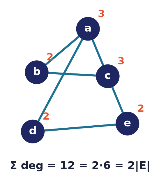
Theorem 10.1 (Handshaking Lemma). In any graph (simple or multi),
Proof. We count in two ways the set
of incidences — vertex–edge pairs in which the vertex is an endpoint of the edge. This is the classic double-counting technique.
Count by vertices. Group the incidences by their first coordinate. A fixed vertex appears in exactly incidences, one for each edge at (a loop at produces two incidences — one for each end — matching the “counts twice” convention). Hence
Count by edges. Group the incidences by their second coordinate. A fixed edge has exactly two endpoints, so it appears in exactly two incidences (for a loop, the two endpoints coincide but the two incidences are still counted). Hence
Equating the two expressions for the same quantity gives .
The lemma is often phrased for a party: the total number of hands shaken (summed over people) is twice the number of handshakes, since each handshake involves two hands. Its most-used consequence is a parity statement.
Corollary 10.2 (odd-degree vertices). In any graph, the number of vertices of odd degree is even.
Proof. Partition the vertices by the parity of their degree:
By Theorem 10.1,
The right-hand side is even. The sum is a sum of even numbers, hence even. Subtracting, is even. But this is a sum of odd numbers, and modulo each odd number is , so
Thus is even.
Remark. What rules out the Königsberg walk (§10.1) is the even-degree condition for an Eulerian circuit: a closed walk that uses every edge exactly once must pair the edges at each vertex into an entry and an exit, so every vertex must have even degree. Königsberg’s graph has four odd-degree vertices, violating this, so no such walk exists. Note that Corollary 10.2 is not violated here — four is an even number of odd-degree vertices, so the graph is perfectly consistent; the obstruction is the even-degree requirement itself, not the parity of the count of odd vertices. Corollary 10.2 does, however, instantly answer questions like “can people each shake hands with exactly others?” — no, because that would be vertices of odd degree , an odd count.
Proposition 10.3 (directed handshaking). In any digraph ,
Proof. Every arc has exactly one tail and one head . Summing out-degrees counts each arc once, at its tail; summing in-degrees counts each arc once, at its head. Both totals therefore equal the number of arcs, .
A second, less obvious counting consequence uses the pigeonhole principle (Lecture 8).
Proposition 10.4 (two vertices of equal degree). Every simple graph with vertices has two distinct vertices of the same degree.
Proof. In a simple graph each degree lies in , a set of possible values. Suppose, for contradiction, that all vertices had distinct degrees; then every value would occur exactly once. In particular some vertex has degree (isolated, adjacent to nobody) and some vertex has degree (adjacent to all other vertices, hence adjacent to ). This contradicts being isolated. So not all values can occur, leaving at most distinct degrees for vertices; by pigeonhole two vertices coincide in degree.
Example (degrees and Handshaking in ). In the running graph :
| vertex | incident edges | |
|---|---|---|
The degree sequence is , whose sum is . Indeed , confirming Theorem 10.1, and has exactly two odd-degree vertices ( and ) — an even count, as Corollary 10.2 requires. There are no isolated vertices, and (illustrating Proposition 10.4) the degree repeats three times.
Example (digraph degrees). Take the digraph on with arcs . Then ; ; . The out-degrees sum to , the in-degrees sum to , and , illustrating Proposition 10.3.
10.5 Special families of graphs
Certain graphs recur so often that they have standard names and formulas.
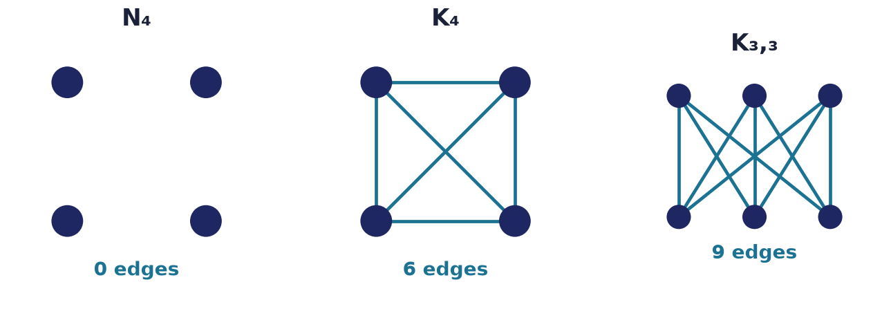
- Null (empty) graph . The graph on vertices with no edges at all: . Every vertex is isolated and . It is -regular.
- Path . vertices in a line with edges ; it has edges, two pendants (the ends), and all interior vertices of degree .
- Cycle (). vertices arranged in a ring: edges . It has edges and is -regular.
- Complete graph . A simple graph on vertices in which every pair of distinct vertices is joined by an edge. It is -regular.
- Complete bipartite graph . The vertex set splits into two disjoint parts ( vertices) and ( vertices); every vertex of is joined to every vertex of , and there are no edges inside a part. A graph whose vertices split into two such edge-free parts is bipartite; is the largest bipartite graph on those parts. The special case is a star.
Theorem 10.5 (edge counts).
Proof. has no edges by definition.
For we give two proofs. (i) Bijective. In a simple graph an edge is a -element subset of ; in every such subset is present, so the edges are in bijection with the -subsets of an -set, of which there are . (ii) Via Handshaking. Every vertex of has degree , so by Theorem 10.1,
For , group the edges by their endpoint in . Each of the vertices of is joined to all vertices of and to no others, contributing exactly edges, and no edge is counted twice (each edge has exactly one endpoint in ). Hence . Equivalently, by Handshaking every vertex of has degree and every vertex of has degree , so .
Theorem 10.6 (maximum size of a simple graph). A simple graph on vertices has at most edges, with equality iff it is .
Proof. Its edge set is a set of distinct -subsets of the -element set (distinct because there are no parallel edges; -subsets because there are no loops). There are only such subsets in all, so . Equality holds iff every -subset is an edge, which is precisely the definition of .
Example. A round-robin tournament among players, where everyone plays everyone once, is modelled by : games. A recommendation setting with users each able to rate any of movies is modelled by : possible user–movie edges, and no user–user or movie–movie edges. Numerically, (a triangle) has edges, has , has , and has .
Remark (density). Theorem 10.6 says a simple graph has edges. A graph with edges is called dense; one with edges is sparse. The distinction drives the choice of data structure in Lecture 11: adjacency matrices favour dense graphs, adjacency lists favour sparse ones.
10.6 Matrix representations
Graphs are convenient for humans to draw, but a computer needs a numeric encoding. The two standard ones are the adjacency matrix and the incidence matrix.
Adjacency matrix
The adjacency matrix of a graph on vertices is the matrix with
For a simple graph every entry is or . Key properties: for an undirected graph is symmetric (); the diagonal is when there are no loops (a loop at contributes to in the usual convention — though some worksheets, e.g. Practical 5, instead record the number of loops on the diagonal, counting a loop once); and the -th row sum equals . For a digraph, when the arc is present, so need not be symmetric; the row sum gives and the column sum gives .
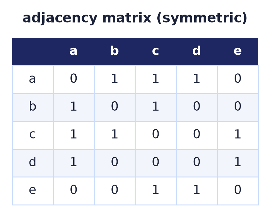
Example. Ordering the vertices , the adjacency matrix of the running graph is:
| 0 | 1 | 1 | 1 | 0 | |
| 1 | 0 | 1 | 0 | 0 | |
| 1 | 1 | 0 | 0 | 1 | |
| 1 | 0 | 0 | 0 | 1 | |
| 0 | 0 | 1 | 1 | 0 |
It is symmetric across the diagonal, the diagonal is all (no loops), and the row sums reproduce the degree sequence found earlier.
What the powers of count
The single most useful algebraic property of the adjacency matrix is that its powers count walks. As defined in §10.8, a walk of length from to is a sequence of edges with each consecutive pair adjacent; vertices and edges may repeat.
Theorem 10.7 (walk counting). Let be the adjacency matrix of a graph (directed or undirected) on . For every integer , the entry of equals the number of walks of length from to .
Proof. By induction on .
Base . We take , the identity. A walk of length is a single vertex with no edges; there is exactly one such walk from to when (the trivial walk) and none when . This matches , which is if and otherwise. (The case is also immediate: , and is by definition the number of length- walks — i.e. edges — from to .)
Inductive step. Assume the claim for some : is the number of walks of length from to , for all . Since , the definition of matrix product gives
Interpret the right-hand side combinatorially. Every walk of length from to is obtained uniquely by taking a walk of length from to some vertex and then appending one edge from to ; the vertex is exactly the second-to-last vertex of the walk. Conversely each such pair (a length- walk to , plus an edge ) yields a distinct length- walk. So, summing over the possible ,
using the induction hypothesis in the last step and the fact that is the number of edges (length- walks) from to . This equals , completing the induction.
Example. Squaring the adjacency matrix of gives
| 3 | 1 | 1 | 0 | 2 | |
| 1 | 2 | 1 | 1 | 1 | |
| 1 | 1 | 3 | 2 | 0 | |
| 0 | 1 | 2 | 2 | 0 | |
| 2 | 1 | 0 | 0 | 2 |
Reading off entries of :
- : there are two walks of length from to , namely and .
- : no length- walk from to (their neighbourhoods and are disjoint), even though is an edge (a length- walk).
- The diagonal entries equal the degrees. This is no accident: a closed walk of length from goes to a neighbour and back, so in a simple graph.
Remark (counting triangles). By the same theorem the diagonal of counts closed walks of length . Each such walk is a triangle traversed from one of its three vertices in one of two directions, so is twice the number of triangles through , and
For one computes , correctly detecting its single triangle . This is the theoretical basis of matrix-based triangle-counting used in network analysis.
Common pitfall. counts walks, not paths or trails — repeated vertices and edges are allowed. Counting paths of a given length is a much harder problem (no simple matrix formula), and conflating the two is a frequent error.
Incidence matrix
The incidence matrix has one row per vertex and one column per edge; if vertex is an endpoint of edge , and otherwise. In a simple graph every column has exactly two $1$s (an edge has two endpoints), and the -th row sum equals again. A loop is the exceptional case, encoded by a single in its column.
Example. Label the edges . The incidence matrix of is:
| 1 | 1 | 1 | 0 | 0 | 0 | |
| 1 | 0 | 0 | 1 | 0 | 0 | |
| 0 | 1 | 0 | 1 | 1 | 0 | |
| 0 | 0 | 1 | 0 | 0 | 1 | |
| 0 | 0 | 0 | 0 | 1 | 1 |
Each column sums to (illustrating the Handshaking double count column by column: summing all entries gives ), and the row sums are once more the degrees.
Remark (which representation?). The adjacency matrix is compact () and answers “are adjacent?” in ; the incidence matrix () records the vertex–edge structure explicitly and generalises cleanly to multigraphs and (with entries, tail and head ) to digraphs, where it underlies flow and circuit theory. In practice large sparse graphs are stored as adjacency lists (each vertex keeps a list of its neighbours), the workhorse representation for the algorithms of Lecture 11.
10.7 Weighted graphs
A weighted graph is a graph together with a weight function assigning a number — a cost, length, capacity, or time — to each edge. (Digraphs may be weighted the same way.) The weight of a walk is the sum of the weights of the edges it uses. Weighted graphs are what make questions like “shortest route” or “cheapest network” meaningful; the algorithms that answer them (Dijkstra, Bellman–Ford, Prim, Kruskal) belong to Lecture 11, but the model belongs here.
In a computer we store weights by replacing the $1$s of the adjacency matrix with the weight , using a sentinel such as (or a separate boolean mask) for “no edge”.
Example. Model four cities with road lengths in kilometres: . The route has weight km, whereas has weight km, so the second route is shorter even though it uses fewer edges. The weight, not the number of edges, is what we minimise — a distinction that separates “fewest hops” (unweighted shortest path, solved by breadth-first search) from “shortest distance” (weighted shortest path, solved by Dijkstra), both in Lecture 11.
10.8 Walks, trails, paths, circuits, and cycles
Movement through a graph is described by walks, which are then refined by forbidding repetition of edges or vertices.
A walk of length is an alternating sequence of vertices and edges
in which each edge joins and . Its length is the number of edges, . In a simple graph a walk is determined by its vertex list, so we write it as . The endpoints are (start) and (end).
- A walk is closed if it starts and ends at the same vertex (), and open otherwise.
- A trail is a walk with no repeated edge (vertices may repeat).
- A path is a walk with no repeated vertex (hence no repeated edge either).
- A circuit is a closed trail: it returns to its start and repeats no edge.
- A cycle is a closed path: it returns to its start and repeats no vertex except that final return. A cycle of length is a copy of ; the shortest cycle in a simple graph has length (a triangle). The length of a shortest cycle is the girth.
The containment hierarchy is: every path is a trail, and every trail is a walk; every cycle is a circuit, and every circuit is a closed walk. The reverse inclusions fail, as the examples below show.
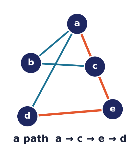
Example (from the running graph ).
- uses edges — all distinct, so it is a trail; but vertex repeats, so it is not a path. Its start and end differ, so it is an open walk of length .
- uses edges — all distinct and it returns to , so it is a circuit. No interior vertex repeats, so it is in fact a cycle of length (a ).
- never repeats a vertex, so it is a path (open, length ).
The next theorem is the workhorse behind every connectivity argument: whenever vertices are joined by any walk, they are joined by a genuine path.
Theorem 10.8 (walk implies path). If a graph contains a walk from to , then it contains a path from to .
Proof. The set of walks from to is non-empty by hypothesis, and each has a length in , so by well-ordering we may choose a walk
of minimum length . We claim repeats no vertex, so that it is a path. Suppose instead that for some . Then
is again a walk from to : the splice is legal because is adjacent to (that edge was in ). But has length , contradicting the minimality of . Hence no vertex repeats and is a path.
Remark. Theorem 10.8 lets us use “walk” and “path” interchangeably when we only care about reachability, which is why the definition of connectivity in §10.9 can be stated with either word.
Example (a cycle from minimum degree). Here is a small argument of the flavour you will meet in the exercises: if every vertex of a finite simple graph has degree , then the graph contains a cycle. Take a longest path . Since , the vertex has a neighbour other than . If were outside , we could prepend it to get a longer path, contradicting maximality; so for some , and is a cycle.
10.9 Connectivity
A graph is connected if there is a walk (equivalently, by Theorem 10.8, a path) between every pair of vertices; otherwise it is disconnected and falls apart into maximal connected pieces called connected components. To make “pieces” precise:
Proposition 10.9 (components as equivalence classes). Define a relation on by iff there is a walk from to . Then is an equivalence relation, and its classes are exactly the vertex sets of the connected components.
Proof. We check the three axioms (Lecture 3). Reflexive: the length- walk joins to itself, so . Symmetric: reversing a – walk yields a – walk, so (edges are undirected). Transitive: concatenating a – walk with a – walk yields a – walk, so and . Thus partitions ; each class is connected (any two of its members are joined by a walk) and maximal (no vertex outside is reachable), which is the definition of a component.
The running graph is connected — for instance reaches via . Adding an isolated vertex would make the graph disconnected, with two components and .
Bridges and cut vertices. An edge whose removal increases the number of components is a bridge; a vertex whose removal (with its incident edges) does so is a cut vertex. In , the edge is not a bridge (the cycle provides an alternate route), whereas in a path every edge is a bridge. These notions measure how robustly a network stays connected — directly relevant to fault-tolerant network design.
For digraphs one distinguishes strong connectivity (a directed path both from to and from to , for every pair) from weak connectivity (the underlying undirected graph is connected). The web link graph, for example, is at best weakly connected: you can often follow links from page to page without any return route. Systematic algorithms for finding components and testing connectivity (BFS/DFS, Tarjan’s strongly-connected-components algorithm) are covered in Lecture 11.
10.10 Graph isomorphism and invariants
Two drawings can look completely different yet represent the same graph. We capture “same structure” precisely.
Two graphs and are isomorphic, written , if there is a bijection that preserves adjacency both ways:
Such an is an isomorphism. Intuitively, relabels the vertices of to turn it into without adding or deleting any edge. Isomorphism is an equivalence relation on graphs (identity, inverse, and composition of isomorphisms are isomorphisms), so it sorts all graphs into isomorphism classes; “the” cycle or “the” graph really means one such class.
How to argue two graphs are isomorphic: exhibit an explicit bijection and check that every edge of maps to an edge of and vice versa. Because is a bijection on finite vertex sets of equal size, it suffices to check that maps every edge to an edge and (the reverse direction then follows by counting).
How to argue they are not isomorphic: find a graph invariant — a quantity or property preserved by every isomorphism — on which the two graphs differ. If a single invariant differs, no isomorphism can exist.
Proposition 10.10 (degree sequence is an invariant). If is an isomorphism, then for every vertex ; consequently and have the same degree sequence.
Proof. Fix . The map restricts to a function from to : if then , so , i.e. . This restriction is injective (as is) and surjective onto (any neighbour of is for the unique , and ). Hence , i.e. . Applying to all vertices reorders the degree list without changing it.
Other convenient invariants: the order , the size , the number of connected components, the girth and the multiset of cycle lengths, the number of triangles (), and whether the graph is bipartite.
Common pitfall. Invariants are necessary but not sufficient: matching degree sequences (or even all of the invariants above) do not guarantee isomorphism. The next example makes this concrete.
Example (isomorphic — pentagon vs. pentagram). Draw once as a regular pentagon with edges and once as a five-pointed star (pentagram) with edges . Define by
Check each pentagon edge maps to a star edge: , , , , . All five images are star edges and is a bijection, so the pentagon and pentagram are isomorphic — both are .
Example (not isomorphic — different degree sequence). Let be the running graph with degree sequence and with degree sequence . Both have vertices, but has edges to ’s , and their degree sequences differ, so (either invariant alone suffices).
Example (not isomorphic — same degree sequence). Consider two -regular graphs on vertices: the cycle , and the disjoint union of two triangles. Both have vertices, edges, and degree sequence — every “local” invariant agrees. Yet they are not isomorphic: is connected (one component) while has two, and isomorphism preserves the number of components. Equivalently, has girth and no triangle, whereas has girth and two triangles.
Example (not isomorphic — both connected, same degree sequence). There are exactly two -regular simple graphs on vertices, and this pair is the classic warning. Both have vertices, edges, degree sequence , and both are connected:
- — bipartite, hence triangle-free (girth ).
- the triangular prism (two triangles joined by a matching, i.e. ) — which contains triangles (girth ).
Since “number of triangles” (equivalently “is bipartite”) is an invariant and the two graphs differ on it, prism, even though every degree-based test is fooled. This is exactly why “same degree sequence” can never prove isomorphism.
Remark (the isomorphism problem). Deciding whether two graphs are isomorphic is a famous problem whose exact complexity is still open: no polynomial-time algorithm is known, yet it is not known to be NP-complete either (Babai’s 2016 algorithm runs in quasipolynomial time). In practice one prunes with cheap invariants first and searches for the bijection only when they all match.
10.11 Planar graphs and Euler’s formula
A graph is planar if it can be drawn in the plane so that no two edges cross (edges meet only at shared endpoints). Such a crossing-free drawing is a plane graph. A plane graph divides the plane into faces (maximal connected regions), including one unbounded outer face. The boundary walk of a face traverses the edges around it; the number of edge-steps in that walk is the degree of the face, where a bridge is counted twice (the walk runs along both of its sides).
Note the distinction: planar is a property of the abstract graph (a drawing exists); plane refers to a specific crossing-free drawing. A planar graph has many plane drawings, but Euler’s formula shows they all share the same face count.
Theorem 10.11 (Euler’s formula, 1750s). For every connected plane graph with vertices, edges, and faces,
Proof. Induction on the number of edges .
Base case . A connected graph with no edges has exactly one vertex, so . Its drawing occupies the plane with a single (outer) face, so . Then .
Inductive step. Let and assume the formula holds for every connected plane graph with fewer than edges. Let be a connected plane graph with edges, vertices, faces. Two cases.
Case 1: contains a cycle. Pick an edge that lies on a cycle. A cycle drawn in the plane is a closed curve which, by the Jordan curve theorem, separates the plane into an inside and an outside; the two sides of therefore lie in two different faces. Delete . Its two adjacent faces merge into one, so the face count drops by exactly ; the vertex count is unchanged; and stays connected, because any route that used can instead go the other way around the cycle. The resulting plane graph has , , . By the induction hypothesis,
Case 2: contains no cycle (it is a tree). A finite tree with at least one edge has a vertex of degree : follow a longest path; its final vertex has no neighbour off the path (that would extend the path) and no second neighbour on it (that would close a cycle), so . Delete and its single incident edge . Being a bridge lying inside a single face, borders the same face on both sides, so deleting it does not change the face count; it removes one vertex and one edge, and leaves connected. Thus , , . By the induction hypothesis,
In both cases , completing the induction.
Remark (topological facts used). The proof leans on two intuitively obvious but genuinely topological facts — that a cycle separates the plane (Jordan curve theorem) and that a bridge borders one face on both sides. A fully rigorous treatment of these belongs to topology; at this level we take them as given, as Rosen and West do.
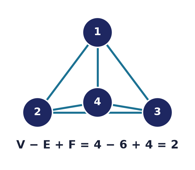
Example. is planar: drawn without crossings (a triangle with a vertex in the middle joined to all three) it has , , and (three inner triangular regions plus the outer face), and indeed .
The real power of Euler’s formula is the edge bounds it forces on planar graphs, which give a quick non-planarity test.
Corollary 10.12 (edge bound). In a simple connected planar graph with ,
Proof. Fix a plane drawing with faces. In a simple graph with and at least two edges, every face has degree : a face of degree would need a loop and a face of degree would need parallel edges (or the whole graph to be a single edge, excluded by ), both forbidden. Now count edge–face incidences: summing the degrees of all faces counts each edge exactly twice (an edge borders two faces, or is a bridge counted twice on the one face it touches), so
Since each of the terms is at least , we get , i.e. . Substitute from Euler’s formula:
Corollary 10.13 ( is not planar). The complete graph is non-planar.
Proof. is simple and connected with and . If it were planar, Corollary 10.12 would give , i.e. — false. Hence is not planar.
The bound does not settle , which has , and . We need a sharper bound exploiting the absence of triangles.
Corollary 10.14 (triangle-free bound). In a simple connected planar graph with and no triangles (girth ),
Proof. With no triangles, every cycle — hence every face boundary — has length , so every face has degree . As before , giving , i.e. . Substituting :
Corollary 10.15 ( is not planar). The complete bipartite graph is non-planar.
Proof. is simple, connected, and bipartite, so it has no odd cycle and in particular no triangle; it has and . If it were planar, Corollary 10.14 would give , i.e. — false. Hence is not planar.
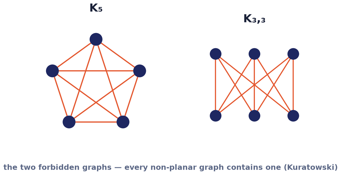
These two graphs are the “three utilities” puzzle (: connect three houses to gas, water, and electricity without crossing pipes — impossible) and the “five mutually connected points” graph (). Kuratowski proved they are the only essential obstructions to planarity.
Theorem 10.16 (Kuratowski, 1930). A graph is planar if and only if it contains no subgraph that is a subdivision of or of .
Here a subdivision of a graph is obtained by repeatedly replacing an edge with a path through new degree- vertices (placing extra points along an edge). Subdividing does not change whether a graph can be drawn without crossings, so a hidden or — even stretched out with extra vertices along its edges — forces non-planarity, and its absence guarantees planarity. (We do not prove Kuratowski’s theorem; the “only if” direction is what Corollaries 10.13 and 10.15 establish for the two base cases, and the “if” direction is deep.) A closely related characterisation, Wagner’s theorem, replaces “subdivision” by “minor”.
Remark (CS relevance). Planarity is not just recreational. Planar graphs can be tested and drawn in linear time (Hopcroft–Tarjan), they admit small separators enabling divide-and-conquer, and they arise directly in VLSI chip layout (wires must not cross on a layer) and in geographic and circuit maps.
10.12 Graph colouring
A proper vertex colouring assigns a colour to each vertex so that adjacent vertices receive different colours. The chromatic number is the minimum number of colours in a proper vertex colouring. Applications include scheduling (colours = time slots, edges = conflicts, so a proper colouring is a conflict-free timetable), examination timetabling, frequency assignment, and register allocation in compilers (colours = CPU registers, edges = variables simultaneously live).
Lower bounds. If contains a clique of size (a copy of , i.e. mutually adjacent vertices), then those vertices need distinct colours, so . Writing for the largest clique size, .
An upper bound. : colour the vertices one at a time in any order, always choosing the smallest colour not yet used on an already-coloured neighbour. When a vertex is coloured it has at most earlier neighbours, so one of the colours is always free. (This greedy procedure and its analysis as an algorithm are developed in Lecture 11; here we use it only to bound .)
Basic values. (no edges, one colour suffices); (all vertices mutually adjacent, so , and colours clearly suffice). The next theorem pins down the graphs colourable with two colours.
Theorem 10.17 (2-colourable = bipartite = no odd cycle). For any graph the following are equivalent: (i) ; (ii) is bipartite; (iii) has no cycle of odd length.
Proof. (i) (ii). A proper -colouring with colours is exactly a partition of into $X={$colour and $Y={$colour with no edge inside or inside — which is the definition of bipartite. (An edgeless graph is bipartite and -colourable, still .)
(ii) (iii). Suppose is bipartite with parts , and let be any cycle. Consecutive vertices are adjacent, hence lie in opposite parts, so the vertices alternate along the cycle. Returning to the start after steps forces into the same part as , which requires an even number of alternations, i.e. even. So every cycle has even length; no odd cycle exists.
(iii) (ii). Suppose has no odd cycle. Colour each component separately (a disjoint union of bipartite graphs is bipartite), so assume connected. Fix a root and let be the length of a shortest path from to . Put and . We claim no edge joins two vertices of the same part. Suppose were such an edge with, say, and of equal parity. Take shortest paths from to and from to ; walking along , across the edge , and along is a closed walk of length , which is odd because is even. A closed walk of odd length must contain a cycle of odd length (repeatedly excising even closed sub-walks between repeated vertices cannot destroy the odd parity, and eventually leaves a cycle) — contradicting the hypothesis. Hence every edge joins to , and is bipartite.
Corollary 10.18 (cycles). An even cycle has ; an odd cycle has .
Proof. has no odd cycle (its only cycle has even length ), so by Theorem 10.17 it is -colourable, and it has an edge so ; thus . is itself an odd cycle, so by Theorem 10.17 , i.e. ; and colours suffice (colour around the cycle , giving the last vertex the spare colour ). Thus .
A proper edge colouring assigns a colour to each edge so that edges sharing a vertex receive different colours; the minimum number needed is the chromatic index .
Proposition 10.19 (edge-colouring lower bound). .
Proof. The edges incident with a maximum-degree vertex pairwise share that vertex, so they must all receive different colours.
Remarkably, this lower bound is almost always tight.
Theorem 10.20 (Vizing, 1964). Every simple graph satisfies
Vizing’s theorem is difficult and we do not prove it; graphs attaining the lower value are called class 1 and those needing are class 2.
Remark (multigraphs). Vizing’s bound is for simple graphs. If parallel edges are allowed, can exceed : Vizing’s multigraph bound is , where is the largest edge multiplicity. A matching-based lower bound is , since each colour class is a matching of at most edges. (Practical 5 uses both bounds on a multigraph.)
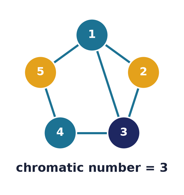
Example (vertex colouring of ). The running graph contains the triangle , a clique of size , so by the clique bound. Three colours suffice: take , then (its only coloured neighbour is ) and (neighbours , ). Every edge now joins differently coloured vertices, so .
Example (chromatic number vs. index differ). The -vertex Petersen graph is -regular () with and . It shows two things at once: colouring vertices and colouring edges are genuinely different problems, so and need not be equal; and a class- graph exists where Vizing’s upper bound is attained. Constructing an optimal colouring (as opposed to knowing its size) is the algorithmic question of Lecture 11.
Remark (Four Colour Theorem). Every planar graph is -colourable — the celebrated Four Colour Theorem, conjectured in 1852 and finally proved by Appel and Haken in 1976 with substantial computer assistance, the first major theorem so proved. It says any political map can be coloured with four colours so that neighbouring regions differ, since the “adjacency graph” of a map is planar.
The chromatic polynomial
Beyond the minimum number of colours, one can count how many proper colourings a graph has. The chromatic polynomial is the number of proper vertex colourings of using at most colours; is then the smallest with . It is computed by deletion–contraction: for any edge ,
where deletes and contracts it (merges ) — colourings of that give the same colour are exactly the colourings of , so subtracting removes the improper ones. Base cases: the empty graph has ; a tree on vertices has ; the complete graph has ; and a cycle has . That is always a polynomial in is itself a theorem (immediate from the recurrence by induction on edges).
Subgraphs, revisited
Recall (§10.3) that is a subgraph of if and . Two special kinds recur: an induced subgraph keeps a vertex subset together with every edge of between them (cliques and independent sets are induced subgraphs); a spanning subgraph keeps all vertices () and only some edges (a spanning tree is the key example, Lecture 12). Monotone parameters respect the containment: deleting edges or vertices cannot raise , , or the maximum degree.
Chapter summary
- A graph pairs vertices with unordered edges; a digraph uses ordered arcs. Simple graphs forbid loops and parallel edges. Order , size .
- Core terms: adjacent vertices, incident vertex–edge pairs, degree (with in-/out-degree for digraphs), isolated vertices, pendants, , , -regular.
- Handshaking Lemma (Thm 10.1): , by double-counting incidences. Corollary 10.2: the number of odd-degree vertices is even. Digraph version (Prop 10.3): . Prop 10.4: any simple graph on vertices has two vertices of equal degree.
- Edge counts (Thm 10.5): , ; a simple graph has at most edges, uniquely maximised by (Thm 10.6).
- Representations: the symmetric adjacency matrix (row sums = degrees) and the incidence matrix (column sums ). Thm 10.7: counts walks of length from to (proved by induction); the diagonal of gives degrees and . Weighted graphs attach a cost to each edge.
- Movement: walk trail (no repeated edge) path (no repeated vertex); closed versions are circuit (closed trail) and cycle (closed path). Thm 10.8: a walk from to yields a path.
- Connectivity: a path joins every pair of vertices; “reachable” is an equivalence relation whose classes are the components (Prop 10.9). Digraphs distinguish strong vs weak connectivity.
- Isomorphism: a bijection preserving adjacency. Prove it by exhibiting the map; disprove it via a differing invariant (order, size, degree sequence, # components, girth, # triangles, bipartiteness). Degree sequence is an invariant (Prop 10.10) but not a complete one — and the prism share it yet differ.
- Planarity: drawable without crossings. Euler’s formula for connected plane graphs (Thm 10.11, induction on edges), giving (Cor 10.12) and, triangle-free, (Cor 10.14); hence (Cor 10.13) and (Cor 10.15) are non-planar. Kuratowski (Thm 10.16): planar iff no subdivision of or .
- Colouring: chromatic number (vertices) and chromatic index (edges). ; ; bipartite no odd cycle (Thm 10.17); and, by Vizing, .
Exercises
Warm-up
-
A graph has vertices, each of degree . How many edges does it have? Explain why no graph can have exactly vertices each of degree .
-
Give the general formula and the number for and .
-
Write the adjacency matrix and the incidence matrix of the path , and verify that the row sums give the degrees and that each incidence-matrix column sums to .
-
Classify each of these walks in the running graph as walk / trail / path / circuit / cycle, and give its length: (i) ; (ii) ; (iii) ; (iv) .
-
Which of the following can be the degree sequence of a simple graph? For each, either draw one or explain the obstruction: (i) ; (ii) ; (iii) ; (iv) .
-
Compute and for , , and . Justify each value.
Standard
-
Prove that in any group of people, at least two people have the same number of friends within the group. (Model as a simple graph and apply Proposition 10.4.)
-
Let be the adjacency matrix of the running graph (§10.6). Using given in the text, state (i) the number of length- walks from to and list them; (ii) the number of length- walks from to , and explain the value; (iii) why the diagonal of reproduces the degree sequence.
-
Decide whether the two graphs below are isomorphic. If they are, give an explicit bijection and verify it on edges; if not, name an invariant that differs. : vertices , edges . : vertices , edges .
-
Exhibit two connected simple graphs on vertices that have the same degree sequence but are not isomorphic, and prove they are not isomorphic.
-
Use the bounds and (where relevant) to decide planarity: (i) ; (ii) ; (iii) the Petersen graph (, , girth ). For those the bounds cannot settle, say so explicitly.
-
A connected planar graph is drawn so that every face (including the outer one) is bounded by exactly edges, and it has vertices. Find and . (Use together with Euler’s formula.)
-
Show that the graph with vertices and edges is not bipartite by exhibiting an odd cycle; then find for it.
-
In a directed graph modelling a round-robin tournament among players (each pair plays once, an arc points from winner to loser), prove that , and deduce the average number of wins.
Challenge
-
Prove that every connected graph on vertices has at least edges. (Hint: induct on , or delete a non-cut edge / contract; relate to trees in Lecture 12.)
-
Reprove the triangle-free bound for a simple connected planar graph with girth and , and use it to give a self-contained proof that is non-planar. Then explain why the same argument does not rule out planarity of .
-
(a) Reproduce the proof that counts walks of length . (b) Prove that a simple graph on vertices is connected iff every entry of is strictly positive. (Hint: entry positive means some walk of length joins ; use Theorem 10.8 to bound path lengths by .)
-
Prove that a finite simple graph in which every vertex has degree at least contains a cycle. (Hint: consider a longest path and its final vertex — see the worked argument at the end of §10.8.)
Selected answers & hints
1. By Handshaking, , so . For vertices of degree : that would be odd-degree vertices, but Corollary 10.2 forces an even number of odd-degree vertices, so it is impossible. (Equivalently is odd, contradicting even.)
3. With order , adjacency matrix rows are , , , ; row sums are the degrees. Edges : each column of the incidence matrix has exactly two $1$s.
4. (i) closed trail with no repeated interior vertex cycle (a triangle, ), length . (ii) no repeated vertex path, length . (iii) reuses the edge , so it is a closed walk but not a trail (hence not a circuit), length . (iv) edges are all distinct and it is open ( to ), with vertex and … note repeats, so it is a trail but not a path, length .
5. (i) yes — the triangle . (ii) sum is odd, so impossible (no graph, simple or not). (iii) sum odd impossible. (iv) sum even; the degree- vertex in a simple graph on vertices must join all others — realisable, e.g. a vertex joined to all, plus one extra edge; yes.
6. : (even cycle, bipartite), . : (odd cycle), (class 2). : (), (colour edges as a proper -edge-colouring of ).
7. Vertices people, edges mutual friendships; this is a simple graph on vertices. By Proposition 10.4 two vertices share a degree, i.e. two people have the same number of friends in the group.
9. Isomorphic — both are -cycles. is ; is the cycle . The bijection carries each edge of to an edge of ; both are .
11. (i) : ; non-planar. (ii) : ; and — bounds are satisfied, so they cannot prove non-planarity, and indeed is planar. (iii) Petersen: girth triangle-free, so — the bound is satisfied and cannot rule out planarity; (Petersen is in fact non-planar, but that requires Kuratowski, not the counting bounds).
12. Every face has degree , so . Euler: . Then , and . (Check: . This is the dodecahedron.)
15. Induct on . For , . For connected, some vertex can be chosen so that has as few components as possible; more simply, take a spanning connected subgraph and delete a leaf of a spanning tree (Lecture 12): each deletion removes one vertex and one edge and preserves connectivity, so .
18. Let be a longest path. Since , has a neighbour . Maximality forbids (else prepend ), so for some , and is a cycle.
Further reading
- K. H. Rosen, Discrete Mathematics and Its Applications — the graph-theory chapters (graphs and graph models, terminology and special graphs, representing graphs and isomorphism, connectivity, Euler and Hamilton paths, planar graphs, graph colouring) closely parallel this lecture and offer many additional worked problems.
- D. B. West, Introduction to Graph Theory — a rigorous, proof-centred treatment; see its chapters on fundamental concepts and degree, trees and distance, planarity (Euler’s formula and Kuratowski’s theorem), and colouring (including Vizing’s theorem).
- Historical background: Euler’s 1736 solution of the Seven Bridges of Königsberg is widely reprinted and discussed in both texts above as the origin of the subject.