Lecture 5. Boolean algebra
5.1 Overview and motivation
Lecture 4 introduced the Boolean domain , the operators (AND), (OR), (NOT), their truth tables, and the basic identities — commutativity, associativity, distributivity, De Morgan, absorption, and the complement laws. We take all of that as known and use it freely. Throughout these notes we write for the complement of (equivalently ), and we use the overline consistently for negation.
That algebra was, in Lecture 4, a set of rules. This lecture puts the rules to work. Every question below is ultimately about cost: a Boolean function can be written in infinitely many equivalent ways, and in hardware each operator we write becomes a physical gate that occupies silicon area, dissipates power, and adds delay. A processor contains billions of gates; shaving one gate off a circuit that is instantiated a million times matters. So the central engineering problem is: given the behaviour we want (a truth table), find the cheapest formula that produces it. This lecture develops the theory and the algorithms that answer that problem.
We proceed through five questions.
- How many functions are there, and how do they relate? — the counting principle and the sixteen functions of two variables.
- How few operators do we need? — functionally complete bases, culminating in the single-gate bases NAND () and NOR (). We prove completeness rigorously.
- How is Boolean algebra realised in hardware? — logic gates, integrated circuits, and translating a formula into a gate network.
- How do we describe a function canonically? — the canonical normal forms (CDNF and CCNF, plus the XOR-based ANF) read off a truth table, proved to exist and to be unique.
- How do we make a formula as small as possible, systematically? — algebraic minimization, Karnaugh maps, and the Quine–McCluskey algorithm, with a cost comparison before and after.
Everything here is combinational: an output depends only on the present inputs, with no memory. Because there are only two truth values, every function of variables is completely described by a finite truth table of rows — a fact we lean on constantly. Adding memory (state that depends on past inputs) turns combinational logic into sequential logic, taken up in Lecture 14 (Automata theory, including Mealy/Moore sequential machines); the minimization techniques here still apply to the combinational “next-state” and “output” blocks inside a sequential machine.
Remark (why this is not just algebra). In Lecture 4 two formulas were “equal” if the identities could transform one into the other. Here we adopt the semantic definition: two formulas are equal iff they have the same truth table. The identities are sound and complete for this semantics (Boolean algebra is complete over ), so the two notions coincide — but the truth-table view is what makes the algorithms below possible, because a truth table is a finite object we can compute on directly.
5.2 Boolean functions and how many there are
Boolean function. A Boolean function of variables is a map
Its domain has points (the rows of a truth table), and to each point it assigns one output bit. Two Boolean functions are equal iff they agree on all inputs.
Because a function is fixed exactly by choosing the output bit for each of the input rows, and each choice is independent with options, we get the fundamental counting principle.
Theorem 5.1 (Counting Boolean functions). There are exactly distinct Boolean functions of variables.
Proof. A function is determined by its output column: a string of bits, one per input row. Distinct output columns give distinct functions (they differ on some row), and every output column arises from some function. Hence functions of variables are in bijection with bit-strings of length , of which there are .
| inputs | functions | |
|---|---|---|
| 0 | 1 | 2 (the constants ) |
| 1 | 2 | 4 () |
| 2 | 4 | 16 |
| 3 | 8 | 256 |
| 4 | 16 | 65 536 |
| 5 | 32 |
The double exponential explodes at once, which is precisely why we do not enumerate functions but reason about them symbolically. For the number is small enough to list in full, and the list is worth memorising because it names every operation we use.
The sixteen functions of two variables
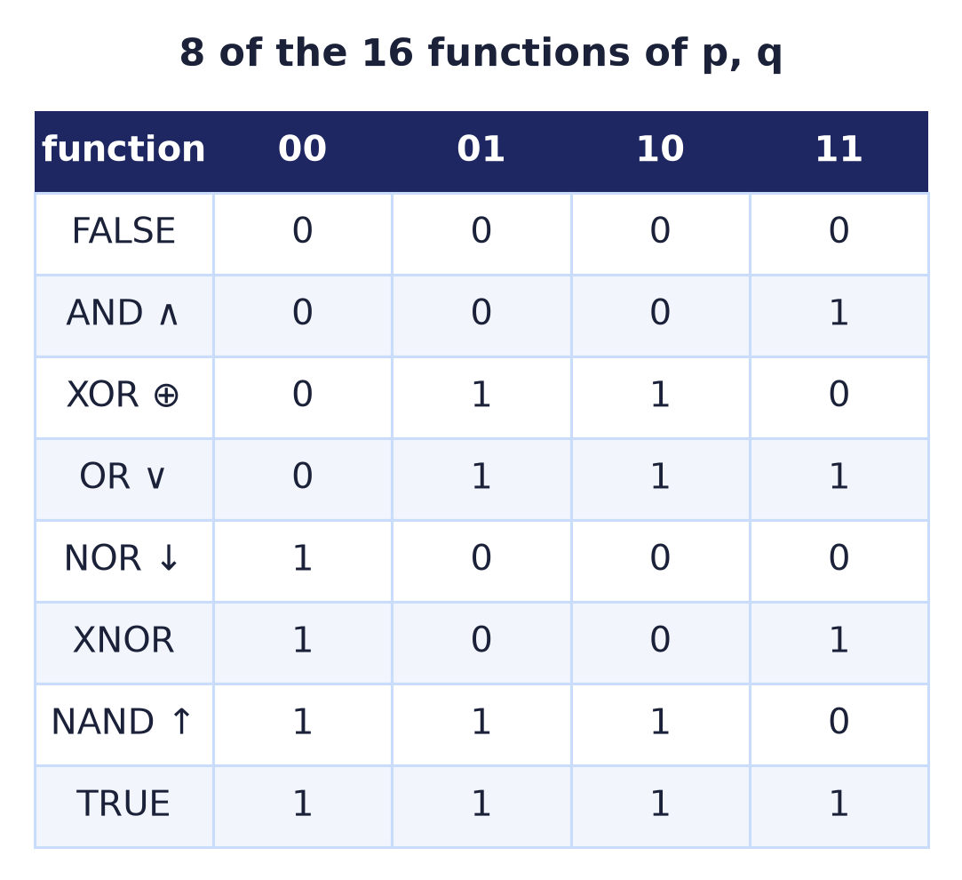
A function of two variables assigns an output to each of the four rows ; there are ways to fill the column, hence 16 distinct two-variable Boolean functions. Reading the output column top-to-bottom for the input order :
| Output | Expression | Name |
|---|---|---|
| 0 0 0 0 | constant false | |
| 0 0 0 1 | AND (conjunction) | |
| 0 0 1 0 | inhibition ( but not ) | |
| 0 0 1 1 | projection / left argument | |
| 0 1 0 0 | inhibition ( but not ) | |
| 0 1 0 1 | projection / right argument | |
| 0 1 1 0 | XOR (exclusive OR) | |
| 0 1 1 1 | OR (disjunction) | |
| 1 0 0 0 | NOR | |
| 1 0 0 1 | XNOR / equivalence | |
| 1 0 1 0 | NOT | |
| 1 0 1 1 | converse implication | |
| 1 1 0 0 | NOT | |
| 1 1 0 1 | implication | |
| 1 1 1 0 | NAND | |
| 1 1 1 1 | constant true |
Notice two distinct symmetries. Complementing every output bit is negation (): it pairs AND NAND, OR NOR, XOR XNOR, , and . Dualization is the separate operation that swaps and (the operational form of the principle of duality from Lecture 4); it pairs AND OR, NAND NOR, and XOR XNOR. Every one of the sixteen can be written with only — which raises the question of how small a set of operators still suffices.
5.3 Functional completeness
Functionally complete set (basis). A set of Boolean operations is functionally complete if every Boolean function, of any number of variables, can be expressed by a formula that uses only operations from (and the input variables).
This is a strong claim — it quantifies over all functions of all arities — so it needs a proof, not a plausibility argument. The cleanest tool is Shannon’s expansion, which peels off one variable at a time.
Theorem 5.2 (Shannon expansion). For any Boolean function and any variable ,
where (the cofactor) is with replaced by the constant .
Proof. Two functions are equal iff they agree on every input, so fix an input and split on the value of . If : the right-hand side is , which is exactly evaluated with . If : it is , exactly with . In both cases the two sides agree, so they are equal as functions.
Theorem 5.3 ( is functionally complete).
Proof. Induction on the number of variables .
Base . The four one-variable functions are , expressible as , , , and respectively — all in the basis.
Inductive step. Assume every function of variables is expressible. Let have variables. By Shannon expansion on ,
Both and have only variables, so by the induction hypothesis each is expressible with . The displayed formula combines them using only , so is expressible too. By induction the claim holds for all .
Iterating the expansion on every variable, and dropping the branches whose cofactor is the constant , produces exactly the sum of minterms (the CDNF of §5.5); Theorem 5.3 is the reason a truth table can always be turned into a formula. From this one result, the smaller bases follow immediately.
Theorem 5.4 ( and are complete).
Proof. By Theorem 5.3 it suffices to rebuild the missing operator. De Morgan gives
so every in a -formula can be rewritten with ; hence is complete. Dually,
shows is complete.
Negation is doing essential work in every one of these bases. Remove it and completeness collapses.
Theorem 5.5 ( is not complete).
Proof. Order the inputs pointwise: for write iff for every . Call monotone if . We show every formula built from (and variables) is monotone, by structural induction:
- a single variable is monotone, since ;
- if are monotone and , then and ; because and are nondecreasing in each argument, and likewise for . So and are monotone.
But negation is not monotone: yet . A non-monotone function therefore cannot equal any -formula, so the set is incomplete.
Common pitfall. Adding the constants does not rescue : the functions and are themselves monotone, and monotone functions are closed under , so still produces only monotone functions and remains incomplete. It is specifically the ability to invert that is missing.
The single-operator bases
Remarkably, one operator can be enough. This is the theoretical justification for building entire chips from a single gate type.
Theorem 5.6 (NAND is complete). The Sheffer stroke alone is functionally complete, via
Proof. We verify each identity, then invoke Theorem 5.3.
- (idempotence ).
- (double negation).
- Using and : (De Morgan).
Thus are each expressible with alone. Since is complete (Theorem 5.3), so is .
Theorem 5.7 (NOR is complete). The Peirce arrow alone is functionally complete, via
Proof. Dual to Theorem 5.6. ; ; and . Each of reduces to , so is complete.
Common pitfall. NAND and NOR are not associative. For instance : taking gives on the left but on the right. So a chain like is ambiguous; always parenthesise, and never assume means (it does not — a -input NAND is a different gate).
Remark (Post’s theorem — the complete picture). Emil Post (1941) classified all complete sets. A set of Boolean functions is complete iff it is not entirely contained in any of the five maximal “clones”: (functions with ), (), (monotone), (self-dual: ), and (affine/linear: ). This gives a slick alternative completeness check for NAND: has , , is non-monotone (), is not self-dual (e.g. ), and equals which is nonlinear (). Lying outside all five classes, is complete — matching Theorem 5.6. NOR fails all five identically.
5.4 Logic gates and circuits
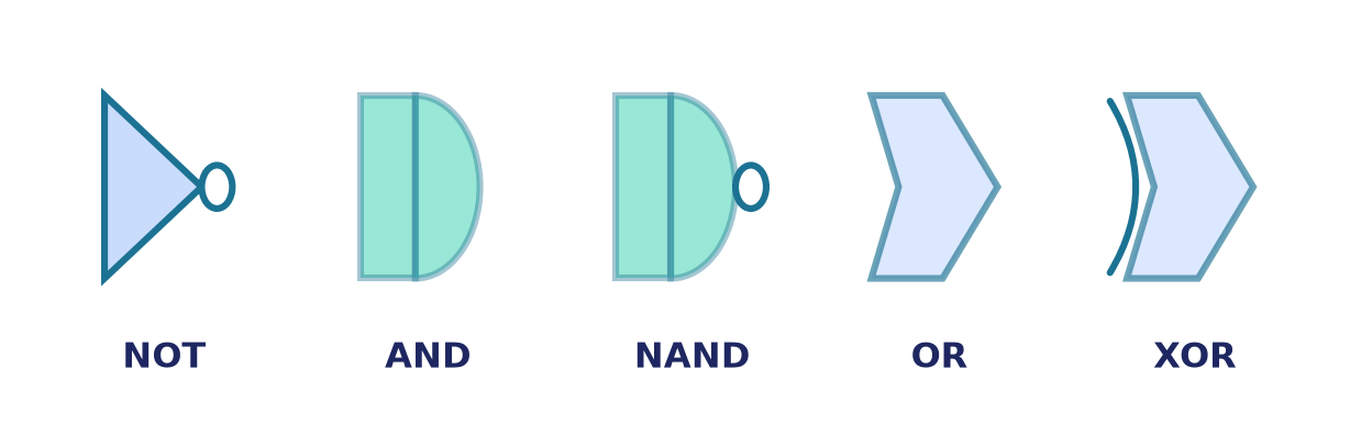
A logic gate is a physical device — today a transistor circuit inside an integrated circuit (IC) — that computes one Boolean operation on its input voltages, interpreting “high” as and “low” as . Gates are the atoms of digital hardware; the abstract algebra of §§5.1–5.3 is exactly the mathematics of what these devices compute. The standard gates, with representative single-gate IC part numbers, are:
| Gate | Function | Symbol shape | Example IC |
|---|---|---|---|
| AND | flat back, round front | SN74LVC1G08-Q1 | |
| OR | curved back, pointed front | SN74LVC1G32-Q1 | |
| NOT (inverter) | triangle + bubble | 7404 | |
| NAND | AND + bubble | SN74AHC1G00 | |
| NOR | OR + bubble | SN74AHC1G02 | |
| XOR | OR + extra back curve | SN74LVC1G86 |
The bubble on a gate symbol always denotes negation, which is why NAND is drawn as AND-with-a-bubble and NOR as OR-with-a-bubble — the pictures encode Theorems 5.6–5.7 visually. Real parts implement these operations directly; larger devices pack many gates to realise a whole function. For example the CY54FCT480T is a dual -bit parity generator/checker — internally a tree of XOR gates, because the parity of a bit-vector is exactly the XOR of all its bits (XOR is associative, so the tree is well defined).
Building a circuit from a Boolean expression
A formula translates mechanically into a gate network: each operator becomes a gate, each variable becomes an input wire, and the wiring follows the nesting of the expression. Complemented inputs are produced by inverters. A sum-of-products (SOP / DNF) formula reads left-to-right as a two-level circuit — a layer of AND gates whose outputs feed a single OR gate — with inverters supplying any complemented literals. Dually, a product-of-sums (POS / CNF) is a layer of ORs feeding one AND.
Take the minimized function (derived in §5.7):
- an inverter produces from ;
- a -input AND gate produces from ;
- a -input OR gate combines and into .
Gate count: NOT AND OR gates.
Everything as NAND (or as NOR)
Because is complete, any two-level AND–OR circuit can be redrawn as an all-NAND network with the same shape. The trick: insert two bubbles (a double negation, hence no change in value) on each wire between the AND layer and the OR layer. The AND gates gain an output bubble and become NANDs; the OR gate gains input bubbles and, by De Morgan (… read the other way, an OR with inverted inputs is a NAND), also becomes a NAND. So:
i.e. AND-then-OR becomes NAND-then-NAND. This is convenient because a board may already carry a NAND package, and because in CMOS a NAND is cheaper than an AND (see §5.9). The takeaway for the rest of the lecture: minimize the algebra first, because every literal and every term you eliminate is gates, transistors, area, delay, and power you never build.
5.5 Canonical normal forms
Minimization needs a well-defined starting point and a way to compare functions. Both are provided by the canonical normal forms: standard expressions built directly from the truth table, one for each function, unique. They are the rigorous bridge between a table and a formula. The two forms below — CDNF and CCNF — are also called the canonical DNF and canonical CNF (the names used in Lecture 6 and Practical 4), or the perfect/complete DNF/CNF; all these names denote the same sum-of-minterms / product-of-maxterms.
- A literal is a variable or its complement ( or ).
- A minterm in variables is a product (AND) of literals, one per variable. Given a point , its minterm is , where and .
- A maxterm is a sum (OR) of literals, one per variable. The maxterm of is (a variable appears complemented where and direct where — the mirror of the minterm rule).
The whole theory rests on one lemma: each minterm switches on exactly one row, each maxterm switches off exactly one row.
Lemma 5.8 (Indicator property). For all : , and .
Proof. Evaluate the literal at : if it is ; if it is . Either way the literal equals iff . The minterm is the AND of all literals, so it is iff every literal is , i.e. iff for all , i.e. iff . Dually, in the literal evaluated at equals iff ; the maxterm is the OR of these, so iff every literal is , i.e. iff for all , i.e. iff .
Corollary 5.9 (Minterms partition the cube). There are exactly minterms, and every input satisfies exactly one of them (namely ). The minterms are the “indicator functions” of the single points.
We use one running example, :
| row # | ||||
|---|---|---|---|---|
| 0 | 0 | 0 | 1 | 0 |
| 0 | 0 | 1 | 1 | 1 |
| 0 | 1 | 0 | 0 | 2 |
| 0 | 1 | 1 | 0 | 3 |
| 1 | 0 | 0 | 1 | 4 |
| 1 | 0 | 1 | 1 | 5 |
| 1 | 1 | 0 | 0 | 6 |
| 1 | 1 | 1 | 1 | 7 |
Canonical disjunctive normal form (CDNF)
CDNF (perfect DNF, sum of minterms). The OR of one minterm for every row where .
Theorem 5.10 (Existence and uniqueness of the CDNF). Every Boolean function equals the disjunction of the minterms of its -rows,
and this is the only way to write as a disjunction of distinct minterms.
Proof. Existence. Let (a nonempty OR since ). For any , by Lemma 5.8 the term contributes iff , and every other minterm is at . Hence , so . Uniqueness. Suppose for some set of minterms. Evaluate at any : by Lemma 5.8 the only term that can be nonzero at is , and it appears iff . So . Therefore is forced — the set of minterms is uniquely determined by .
For our the -rows are (rows ), giving
Indexing minterms by the decimal value of their row, this is written compactly as .
Canonical conjunctive normal form (CCNF)
CCNF (perfect CNF, product of maxterms). The AND of one maxterm for every row where .
Theorem 5.11 (Existence and uniqueness of the CCNF). Every Boolean function equals
and this is the only representation of as a product of distinct maxterms.
Proof. Existence. Let . By Lemma 5.8, exactly when ; so iff some maxterm with has , i.e. iff . Hence . Uniqueness. If , then evaluating at the only factor that can be is , present iff ; so , forcing .
(Equivalently, the CCNF of is obtained from the CDNF of by De Morgan — a one-line derivation once Theorem 5.10 is in hand.)
For our the -rows are (rows ), giving maxterms , , , so
Remark (which form is cheaper). The rows split cleanly: the CDNF uses the -rows, the CCNF uses the -rows, and is all rows. So . A function that is mostly has a long CDNF and a short CCNF, and vice versa — expand around whichever output value is rarer. For our : minterms vs maxterms, so the CCNF is the smaller canonical form.
Common pitfall. The minterm and maxterm polarities are opposite. For a -row, a variable equal to appears uncomplemented in the minterm; for a -row, a variable equal to appears complemented in the maxterm. Getting this backwards is the single most common error in building canonical forms — re-derive it from Lemma 5.8 if in doubt, rather than memorising.
Algebraic normal form (Zhegalkin polynomial)
A third canonical form uses XOR instead of OR. Since is functionally complete, every Boolean function has a unique algebraic normal form (ANF) — a XOR of distinct AND-terms, possibly including the constant :
There are Boolean functions of variables and exactly coefficient vectors — one bit per subset of the variables — and distinct vectors compute distinct functions, so the correspondence is a bijection: every function has exactly one ANF. Equivalently is a polynomial over the two-element field — the Zhegalkin polynomial. Convert any formula to ANF by substituting and , then simplifying with and . The ANF is the natural form for parity and checksums, and a function is affine (linear) exactly when its ANF has degree — the class of Post’s theorem (§5.3).
(De Morgan generalises to any arity, used implicitly when reading a CCNF: and, dually, .)
5.6 Algebraic minimization
The canonical forms are unique but usually far from minimal. Algebraic minimization applies the identities of Lecture 4 to shrink a formula while preserving its truth table. The workhorses are:
| Law | Statement |
|---|---|
| Idempotence | , |
| Complement | , |
| Absorption | , |
| Absorption (2nd form) | |
| Combining / “expand by ” | ; and |
| De Morgan | , |
| Consensus |
The combining law is the algebraic heart of every method in this lecture: two product terms that agree everywhere except in one variable, where they disagree, merge into one shorter term. Karnaugh maps and Quine–McCluskey are just disciplined, exhaustive ways of finding every legal application of this one law.
Quick example (combining + absorption).
The last step is the second absorption form … read as . Three product terms collapse to a single OR.
Consensus example. In , the term is the consensus of and (formed by cancelling the opposed variable ). It is redundant:
so and . Spotting redundant consensus terms is exactly what “don’t add a group you don’t need” means on a Karnaugh map.
Worked example (full derivation). Simplify
| Step | Expression | Justification |
|---|---|---|
| 1 | given | |
| 2 | De Morgan on first term; drop inner parentheses | |
| 3 | double negation | |
| 4 | reorder; multiply by | |
| 5 | distribute | |
| 6 | group with , and with | |
| 7 | complement law | |
| 8 | idempotence ; factor | |
| 9 | absorption (2nd form) with | |
| 10 | drop parentheses |
So .
Remark (the deck’s longer route). The original lecture reached the same answer from step 8 via a chain of De Morgan rewrites: . It is correct but longer; recognising the absorption law (step 9 above) collapses six lines into one. This is exactly why we want systematic methods — algebraic skill varies, and there is no guarantee you spotted the shortest path.
Truth-table check. Building both sides column by column confirms equality (they differ from only where every variable is ):
| (original) | |||||||
|---|---|---|---|---|---|---|---|
| 0 | 0 | 0 | 0 | 1 | 0 | 1 | 1 |
| 0 | 0 | 1 | 0 | 1 | 1 | 1 | 1 |
| 0 | 1 | 0 | 1 | 1 | 0 | 1 | 1 |
| 0 | 1 | 1 | 1 | 0 | 1 | 1 | 1 |
| 1 | 0 | 0 | 0 | 1 | 0 | 1 | 1 |
| 1 | 0 | 1 | 0 | 1 | 0 | 1 | 1 |
| 1 | 1 | 0 | 0 | 1 | 0 | 1 | 1 |
| 1 | 1 | 1 | 0 | 0 | 0 | 0 | 0 |
Algebraic minimization always works, but it gives no guarantee of reaching the smallest form and offers no stopping rule — you can never be sure you are done. This motivates the systematic methods that follow, which do find provably minimal two-level forms.
5.7 Karnaugh maps
A Karnaugh map (K-map) is a truth table redrawn as a grid whose rows and columns are labelled in Gray-code order — successive labels (including the wrap from the last back to the first) differ in exactly one bit. This labelling is the whole point of the map.
Proposition 5.12 (Adjacency = one-variable change). With Gray-code labels, two cells sharing an edge — or lying at opposite ends of the same row or column (wrap-around) — represent inputs that differ in exactly one variable.
Proof sketch. A horizontal move changes only the column label by one Gray-code step, which flips exactly one of the column variables and leaves the row variables (and all other column variables) fixed; a vertical move does the same for the row variables. Gray code is cyclic — for two bits, also differs in one bit — so the first and last positions are one step apart too, justifying wrap-around.
By the combining law, two adjacent -cells differing in variable merge: . Iterating, a block of cells that forms a subcube — chosen variables run through all their combinations while the remaining stay constant — collapses to the single product term of those constant literals.
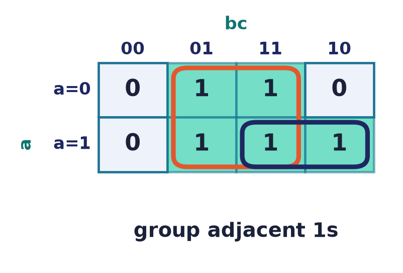
Theorem 5.13 (K-map grouping). A group of cells forming a subcube corresponds to the product term of its constant literals (each constant- variable direct, each constant- variable complemented). This is an implicant of (i.e. , meaning ) iff all cells hold .
Proof. By construction exactly on the cells of the subcube (the free variables are unconstrained, the constant literals pin the rest). Then iff at every point where , i.e. iff all those cells are . The size is a power of two because binary variables range over combinations.
So grouping $1$s into the largest legal subcubes directly reads off short product terms. We formalise the vocabulary:
- An implicant is a product term with .
- A prime implicant (PI) is an implicant from which no literal can be deleted while remaining an implicant — on the map, a group that cannot be enlarged (doubled) and stay all-.
- An essential prime implicant is a PI that covers at least one -cell covered by no other PI.
A minimal SOP is a smallest set of prime implicants that covers every ; it must contain every essential PI, and then a cheapest choice of remaining PIs to cover what is left.
Template layouts (cells left blank):
Two variables — rows , columns :
| 0 | 1 | |
|---|---|---|
| 0 | ||
| 1 |
Three variables — rows , columns in Gray order:
| 00 | 01 | 11 | 10 | |
|---|---|---|---|---|
| 0 | ||||
| 1 |
Four variables — rows , columns , both in Gray order:
| 00 | 01 | 11 | 10 | |
|---|---|---|---|---|
| 00 | ||||
| 01 | ||||
| 11 | ||||
| 10 |
Common pitfall. Do not label the axes (plain binary). Between and two bits change, so plain-binary neighbours are not logically adjacent and the combining law fails. The Gray order is mandatory. Likewise, groups must be rectangles of size a power of two (); an “L-shape” or a -cell group is illegal.
Worked example 1 — a three-variable minimal DNF
Take the running . Rows , columns :
| 00 | 01 | 11 | 10 | |
|---|---|---|---|---|
| 0 | 1 | 1 | 0 | 0 |
| 1 | 1 | 1 | 1 | 0 |
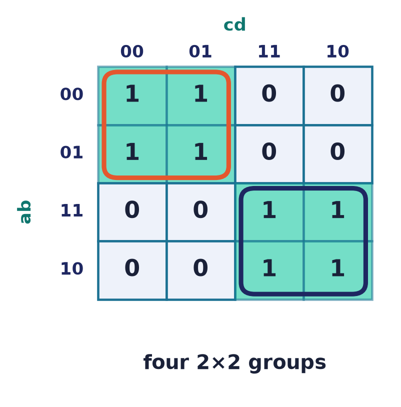
- The left half (columns , both rows) is four adjacent $1$s where only is constant . This is a prime implicant, and it is essential (it is the only cover of the cells at ).
- The two $1$s at and share . Essential, because the cell (minterm ) lies in no other group.
Together they cover every (the cell is shared, which is allowed), giving the minimal DNF
This is dramatically smaller than the five-minterm CDNF and is exactly the expression whose -gate circuit was drawn in §5.4.
Worked example 2 — wrap-around
Let (all even rows). Rows , columns :
| 00 | 01 | 11 | 10 | |
|---|---|---|---|---|
| 0 | 1 | 0 | 0 | 1 |
| 1 | 1 | 0 | 0 | 1 |
The four $1$s sit in columns and — the first and last columns, which are wrap-around adjacent. All four share , so they form one legal group of size :
Without wrap-around one would wrongly split this into two size- groups and then have to combine them algebraically. Wrap-around lets the map find the largest group directly.
Worked example 3 — a four-variable minimal DNF
Consider given by the eight minterms
Plotting each minterm (rows , columns ):
| 00 | 01 | 11 | 10 | |
|---|---|---|---|---|
| 00 | 1 | 1 | 1 | 0 |
| 01 | 0 | 0 | 1 | 0 |
| 11 | 0 | 0 | 0 | 1 |
| 10 | 1 | 1 | 1 | 0 |
Grouping the $1$s into largest subcubes:
- Rows and (wrap-adjacent, both have ) columns (): a block .
- The same two rows () columns (): a block .
- Column , rows (): a vertical pair . (Essential — it is the only cover of the cell .)
- The isolated cell cannot be enlarged (all four neighbours are ), so it stays a full minterm (essential).
Reading a minimal CNF (group the 0s)
For a minimal CNF, group the zeros and read each block as a maxterm — keep the variables constant over the block, complemented where the variable is and direct where it is (Theorem 5.13 with the polarity flipped, because a group of $0$s is a prime implicant of ). The zeros of the same four-variable map:
| 00 | 01 | 11 | 10 | |
|---|---|---|---|---|
| 00 | . | . | . | 0 |
| 01 | 0 | 0 | . | 0 |
| 11 | 0 | 0 | 0 | . |
| 10 | . | . | . | 0 |
Grouping the $0$s:
- Rows () columns (): block, constants .
- Row () columns (): pair .
- Column (), rows (): pair .
- Column (), rows (): pair .
Both readings describe the same function; the DNF form is cheaper when $1$s cluster, the CNF form when $0$s cluster.
Don’t-care conditions
Often some input combinations cannot occur (e.g. the six bit-patterns – that are not valid BCD digits) or their output is simply irrelevant. Such rows are don’t-cares, written (or ). A don’t-care may be treated as or , chosen independently for each group, whichever makes the groups larger. You must still cover every real , but you never have to cover a .
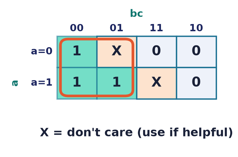
Worked example 4 — BCD “digit ” with don’t-cares. Inputs encode a decimal digit ; patterns – are invalid, hence don’t-cares. iff the digit is , i.e. minterms , with .
| 00 | 01 | 11 | 10 | |
|---|---|---|---|---|
| 00 | 0 | 0 | 0 | 0 |
| 01 | 0 | 1 | 1 | 1 |
| 11 | ||||
| 10 | 1 | 1 |
Using don’t-cares as where helpful:
- The whole bottom half (rows ) can all be (real $1$s at ; the rest are ): a group of .
- Rows () columns (): (covers ; uses at ).
- Rows () columns (): (covers ; uses at ).
Had we forced every don’t-care to , the same function would minimize to
noticeably more expensive. Exploiting don’t-cares is one of the biggest practical wins in logic synthesis.
Remark. A don’t-care is included in a group only if doing so helps; it is never obligatory. Different groups may make opposite assumptions about the same cell — that is fine, because each group is an independent implicant and we only require that the real $1$s are covered and no real is.
Practical rules for K-maps.
- Groups must be rectangular and of size a power of two; wrap-around across all four edges (and the four corners) is allowed.
- Use the largest legal groups (bigger group fewer literals) and the fewest groups that still cover every target cell.
- Identify essential prime implicants first (a that only one group can cover forces that group in), then cover the rest as cheaply as possible.
- Groups may overlap; every (for DNF) or every (for CNF) must lie in at least one group. Don’t-cares may be covered or not, freely.
- K-maps stay readable up to about – variables; beyond that, use the tabular Quine–McCluskey method.
Common pitfall. “Take the largest group first, greedily” does not always give a minimal cover. When no prime implicant is essential (a cyclic chart, see Exercise C3) you must compare competing covers. The map is a visual aid for the reasoning, not a substitute for it.
5.8 The Quine–McCluskey algorithm
Karnaugh maps rely on human pattern-recognition and break down past five variables. The Quine–McCluskey (QM) algorithm (Willard Quine 1952–55, Edward McCluskey 1956) is a fully mechanical procedure that finds all prime implicants and then a minimal cover — it is essentially “the K-map as a table,” suitable for a computer. It has two phases.
Phase 1 — find all prime implicants by repeated combining.
- List all minterms (and don’t-cares) as binary strings; group them by their number of $1$s.
- Compare every string in each group with every string in the next group. If two differ in exactly one bit position, they combine: write a new term with a dash
–in that position, and tick both parents as “used.” - Repeat on the newly formed terms (matching requires the same dash positions and a one-bit difference elsewhere), producing size-, then size- terms, etc., until no more combining is possible.
- Every term never ticked (never absorbed into a larger one) is a prime implicant.
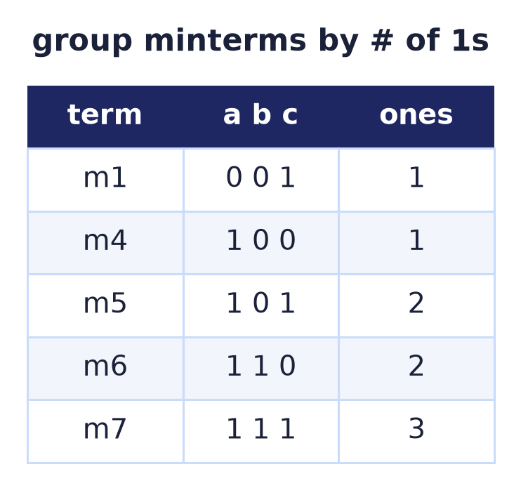
Phase 2 — choose a minimal cover with a prime-implicant chart.
- Build a chart: rows = prime implicants, columns = the original minterms (don’t-cares are not required to be covered, so they get no column). Mark which PI covers which minterm.
- A column with a single mark forces its PI: that PI is essential. Select all essential PIs.
- Delete covered columns; from the remaining PIs choose a minimum-cost subset covering the leftover minterms (by inspection, or Petrick’s method for cyclic charts).
Fully worked example. Minimize .
Phase 1, round 0 — group by number of $1$s:
| Group ($#1$s) | Minterm | |
|---|---|---|
| 0 | 0 | 0000 |
| 1 | 1, 2, 8 | 0001, 0010, 1000 |
| 2 | 10 | 1010 |
| 3 | 11, 14 | 1011, 1110 |
| 4 | 15 | 1111 |
Round 1 — combine adjacent groups differing in one bit (dash the differing position):
| Term | Pattern | from |
|---|---|---|
Every original minterm was used at least once (all ticked).
Round 2 — combine size- terms sharing a dash position and differing in one bit:
| Term | Pattern | from |
|---|---|---|
| and | ||
| and |
The term () never combines further and remains as is; the size- terms cannot combine (different dash patterns). Prime implicants:
| PI | Pattern | Covers | Product term |
|---|---|---|---|
Phase 2 — prime-implicant chart:
| PI \ minterm | 0 | 1 | 2 | 8 | 10 | 11 | 14 | 15 |
|---|---|---|---|---|---|---|---|---|
Reading the single-mark columns: minterm forces ; minterms force ; minterms force . All three PIs are essential, and together they cover — the whole function. Hence
Cross-check on the K-map (rows , cols ):
| 00 | 01 | 11 | 10 | |
|---|---|---|---|---|
| 00 | 1 | 1 | 0 | 1 |
| 01 | 0 | 0 | 0 | 0 |
| 11 | 0 | 0 | 1 | 1 |
| 10 | 1 | 0 | 1 | 1 |
is the four corners (); is the lower-right (); is the pair at the top-left. The tabular method and the map agree, as they must.
Remark (cyclic charts and Petrick’s method). Sometimes no column has a single mark, so there are no essential PIs and the chart is cyclic (see Exercise C3, , where every minterm is covered by exactly two PIs). Then form Petrick’s product , multiply out to SOP using and , and pick the product term with the fewest (cheapest) PIs. This turns “cover the chart” into a Boolean problem itself.
Remark (why QM is not the end of the story). QM finds a minimal two-level SOP, but Phase 2 (the covering problem) is NP-hard in general, so exact QM does not scale to functions with hundreds of variables. Industrial logic synthesis uses the heuristic minimizer Espresso, and moves beyond two-level to multi-level minimization (factoring common subexpressions across many outputs), which is what actually reduces area in a real chip. QM remains the conceptual foundation and the definition of “minimal SOP.”
5.9 Cost: before vs after minimization
Minimization pays off in three currencies: gate count, transistor count (area/power), and delay. Consider again , comparing the raw CDNF against the minimized .
A useful reference for static CMOS (the dominant chip technology): an inverter is transistors; a -input NAND or NOR is transistors; a -input AND is a NAND followed by an inverter, transistors; a -input OR is a NOR plus an inverter, likewise . These figures are approximate but standard, and they explain why NAND/NOR are the “native” gates and AND/OR cost extra.
| Metric | CDNF | Minimized |
|---|---|---|
| Product terms | 5 | 2 |
| Literals | 15 | 3 |
| Inverters (NOT) | 3 (for ) | 1 (for ) |
| AND gates | 5 (three-input) | 1 (two-input) |
| OR gates | 1 (five-input) | 1 (two-input) |
| Gate total | 9 | 3 |
| CMOS transistors (approx.) | ||
| Logic depth (levels) | 2 (+ inverters) | 2 (+ inverter) |
Minimization cuts the gate count by two thirds and the transistor count roughly fourfold, with no loss of speed (both are two-level). Redrawn as NAND-only (§5.4), the minimized circuit is a handful of NAND gates. Multiply such savings across the millions of instances of a standard cell in a modern design and the motivation for §§5.6–5.8 is clear: the algebra is the design, and smaller algebra is a smaller, faster, cooler chip.
Remark (delay). Two-level SOP minimizes logic depth (hence delay) at some cost in width (many wide gates in parallel). Real gates have limited fan-in, so a -input OR is often built from a tree of -input gates, adding depth. Multi-level synthesis trades depth against area to hit a timing target; two-level minimization is the baseline it starts from.
5.10 Historical note and connections
A short history. The algebra of logic is due to George Boole (The Mathematical Analysis of Logic, 1847; An Investigation of the Laws of Thought, 1854), who treated logical reasoning as symbolic calculation. Its application to circuits is due to Claude Shannon, whose 1937 MIT master’s thesis A Symbolic Analysis of Relay and Switching Circuits showed that Boolean algebra exactly describes — and, crucially, simplifies — networks of relays and switches. That single insight founded digital design; the expansion theorem of §5.3 bears his name. The single-operator results are older than the transistor: Charles Sanders Peirce noted around 1880 (unpublished) that one connective suffices, and Henry Sheffer proved it in print in 1913 for the stroke . Emil Post (1941) then classified all complete sets via his lattice of clones. On the minimization side, Edward Veitch proposed a chart in 1952 which Maurice Karnaugh refined into today’s map in 1953 (both at Bell Labs), while Willard Quine (1952, 1955) and McCluskey (1956) gave the tabular algorithm.
Connections to computer science.
- Programmable logic (PLA, PAL): a two-level SOP maps directly onto a programmable AND-plane feeding an OR-plane — minimization literally sets which fuses to blow.
- FPGAs and LUTs: a -input lookup table is a stored truth table, so any -variable function is realised without gate-level minimization at all — a modern echo of Theorem 5.1.
- BDDs: iterating Shannon expansion (Theorem 5.2) with a fixed variable order and sharing identical subfunctions yields the ordered binary decision diagram, the standard data structure for representing and comparing huge Boolean functions in verification.
- SAT and verification: the CNF of §5.5 is the input format for SAT solvers; equivalence checking two circuits reduces to a satisfiability question about their XOR.
- Compilers: short-circuit evaluation, branch simplification, and dead-code elimination apply exactly the identities of §5.6 to program conditions.
- Automata theory (Lecture 14): everything here is combinational (output function of current input). A flip-flop adds state; the machine’s next-state and output logic are combinational blocks minimized by precisely these methods, so this lecture is the foundation of the sequential machines (Mealy/Moore) studied there.
Chapter summary
- A Boolean function is a map ; there are of them, and exactly 16 of two variables (AND, OR, NOT, NAND, NOR, XOR, XNOR, the two implications and inhibitions, the projections, and the two constants).
- Shannon expansion proves is functionally complete by induction; De Morgan then gives completeness of and .
- is not complete — it produces only monotone functions, and is non-monotone. Negation is indispensable.
- NAND () and NOR () are each complete alone: , with two-step rebuilds of and . Post’s theorem characterises all complete sets via five maximal classes.
- Logic gates realise these operations; a formula maps directly onto a gate network, and any two-level AND–OR circuit becomes an all-NAND (or all-NOR) circuit of the same shape.
- CDNF minterms over the -rows and CCNF maxterms over the -rows; both exist and are unique (Theorems 5.10–5.11), read straight from the truth table.
- Algebraic minimization applies the identities (combining, absorption, consensus) — powerful but with no stopping rule.
- A Karnaugh map uses Gray-code labelling so that adjacency one-variable change; grouping $1$s (into power-of-two subcubes, wrap-around allowed, don’t-cares exploited) gives a minimal SOP, grouping $0$s gives a minimal POS. Cover essential prime implicants first.
- Quine–McCluskey mechanises this: combine to find all prime implicants, then use a PI chart (with Petrick’s method for cyclic charts) to pick a minimal cover — scalable past the reach of K-maps.
- Minimization saves gates, transistors, area, power, and delay, which is why it sits at the heart of digital design.
Exercises
Warm-up
W1. How many Boolean functions are there of variables? Of variables? How many of the two-variable functions are monotone?
W2. For the input row , write (a) its minterm and (b) its maxterm.
W3. For , write the CDNF as an expression and the CCNF as a list of maxterms.
W4. Using only NAND gates, build (a) an inverter and (b) a -input AND. Count the gates in each.
W5. Simplify with a single law each: (a) ; (b) ; (c) .
W6. Why must K-map columns be labelled rather than ? Give the two-bit patterns that would become “adjacent” incorrectly.
Standard
S1. Prove that is functionally complete by expressing using only and , and justify each step.
S2. Show that XOR () is not expressible using only . (Hint: monotonicity, or /-preservation.)
S3. Minimize with a K-map. Express the result with a named two-variable operation.
S4. Minimize . (Look before you compute.)
S5. Express using only NOR gates, and count the gates. (Hint: ; or first get from .)
S6. From the truth table of , write both the CDNF and the CCNF, and verify that the index sets and partition .
S7. For the minimized : draw the gate circuit, count gates and (using the §5.9 CMOS figures) transistors, then repeat for a circuit built directly from the five-minterm CDNF. State the ratio.
S8. A four-variable function is on and don’t-care on ; it is elsewhere. Minimize it as an SOP using a K-map, exploiting the don’t-cares.
Challenge
C1. Run Quine–McCluskey on : list all prime implicants, build the PI chart, identify the essential PIs, and give a minimal SOP.
C2. Prove that the minterms of variables partition — i.e. every input satisfies exactly one minterm — and deduce that .
C3. The chart for is cyclic: find all six prime implicants, show the chart has no essential PI, and use Petrick’s method to obtain the (two) minimal SOPs.
C4. Prove that NOR is functionally complete using Post’s criterion — show lies outside each of the five maximal classes .
C5. A function is self-dual if . Prove that a self-dual function of variables has exactly minterms, and that its CDNF and CCNF index sets are complementary “under bit-flip.”
C6. Prove the consensus theorem from the basic identities, and explain what it corresponds to on a Karnaugh map (why the group is redundant).
Selected answers & hints
W1. ; in general . Monotone two-variable functions: — six of them (all the others need negation or are XOR/XNOR).
W2. (a) minterm ; (b) maxterm . Note the opposite polarities.
W3. CDNF . The -rows are , so CCNF .
W4. (a) — one gate. (b) — one NAND for , a second NAND wired as an inverter, so two gates.
W5. (a) ; (b) ; (c) .
S1. : negate each input, OR them, negate the result — De Morgan. Since is complete and is now built from , the smaller set is complete.
S2. is not monotone: but and (fine), yet with . A -formula is monotone (Theorem 5.5), so it cannot be . (Alternatively: every -formula preserves both and , but preserves and not since .)
S3. Group: row (all four $1$s) ; columns (both rows) . So (NAND).
S4. These are exactly the odd rows (LSB ), so . One group of eight; no other literal survives.
S5. Build from (Theorem 5.7) and substitute into ; a compact standard NOR realization of XOR uses five NOR gates. (Any correct all-NOR network is acceptable; count your gates.)
S6. CDNF ; CCNF . The sets and are disjoint and their union is — a partition, as Theorem 5.10/5.11 guarantee.
S7. Minimized: NOT, AND$_2$, OR$_2$ gates, transistors. CDNF: NOT, AND$_3$, OR$_5$ gates, transistors. Ratio about in gates, in transistors.
S8. With the map (rows , cols ) and the don’t-cares at set as convenient, a minimal cover is — set up the map, mark $1$s at and at , and confirm your groups cover all real $1$s while never being forced to cover a . (Multiple minimal answers exist; verify by truth table.)
C1. Essential prime implicants come out to (one correct minimal form) ; build the chart, take every single-mark column’s PI, then cover the rest. Verify your SOP against the minterm list by evaluating all rows.
C2. By Lemma 5.8, ; so for a fixed input , exactly one minterm () is and the other are — the minterms’ -sets are the singletons , which partition . Their OR is therefore on every input: .
C3. Prime implicants: , , , , , . Every minterm is covered by exactly two PIs and every PI covers two minterms — no column has a single mark, so no PI is essential (cyclic). Petrick’s product multiplies out to reveal minimal covers of three PIs each, e.g.
Both use terms / literals.
C4. : ; ; non-monotone since but (); not self-dual, e.g. (); nonlinear, has the degree- term (). Outside all five classes complete by Post.
C5. Pair each input with its bit-complement . Self-duality makes exactly one of each pair a -row, and the inputs split into such pairs, so has exactly minterms. Moreover indexes a minterm (a -row) iff indexes a maxterm (a -row), so the CDNF and CCNF index sets are exact bit-flips of one another.
C6. ; expand ; then and , so is absorbed and drops out, leaving . On a K-map, and are two groups whose union already includes the cells of the group; the group covers nothing new, so adding it only wastes a gate.
Further reading
- K. H. Rosen, Discrete Mathematics and Its Applications — chapter on Boolean algebra (Boolean functions, representing functions, logic gates, minimization, Karnaugh maps).
- Z. Kohavi and N. K. Jha, Switching and Finite Automata Theory — thorough treatment of canonical forms, the Quine–McCluskey algorithm, and multi-output/multi-level minimization.
- C. E. Shannon, “A Symbolic Analysis of Relay and Switching Circuits,” Trans. AIEE 57 (1938) — the founding paper, for historical interest.