Lecture 14. Automata theory
Overview
This is the final topic of the course, and it is where the strands we have been spinning finally braid together. Automata theory is built from sets and tuples (Lecture 2), from functions viewed as a special kind of relation (Lecture 3), from the Boolean/combinational logic of gates and adders (Lecture 5), and from the propositional connectives whose set-theoretic shadows — union, intersection, complement — reappear here as operations on languages (Lecture 6). What is genuinely new is a single idea that none of those earlier chapters possessed: state, a finite memory of the relevant past that lets a device behave differently on the same input depending on where it currently is.
We begin, as the slides do, with a concrete hardware question — the difference between combinational and sequential logic — and then peel away wires and gates until only the essential mechanism remains: a control unit that occupies one of finitely many states and moves between them as it reads symbols. That abstraction is the finite automaton, the central object of this chapter.
From the hardware contrast we build up, in order: the vocabulary of alphabets, strings, and languages; the general abstract machine (tape, reader, control unit); the deterministic finite automaton (DFA) with its extended transition function , its runs, its notion of acceptance, and the language it recognises; the output-producing Mealy and Moore machines; the nondeterministic automaton (NFA) with -moves and the subset construction that flattens it back to a DFA; the identification of finite automata with the regular languages and regular expressions (Kleene) and the closure properties of that class; and finally the pumping lemma, which lets us prove that some languages — famously — lie beyond the reach of any finite automaton. We close with a signpost toward the richer machines (pushdown automata, Turing machines) that lie past the horizon of this course.
Unlike earlier drafts of these notes, this chapter proves what it states. Every theorem comes with a complete argument, and every automaton comes with a trace or an induction that certifies it does what we claim. Deliberately out of scope: Turing machines beyond a mention, and the DFA-minimisation algorithm (Myhill–Nerode is noted but not developed).
14.1 Combinational versus sequential logic
Digital circuits split into two kinds according to what their outputs depend on, and the split is exactly the doorway into automata theory.
Definition (combinational logic). A combinational circuit is one whose outputs are determined only by the current inputs. It has no memory: present the same input bits and you always get the same output bits.
This is precisely the world of Lecture 5. A combinational circuit computes a Boolean function , and everything we said there — truth tables, canonical normal forms, Karnaugh-map minimisation — describes it completely. Typical building blocks are adders, subtractors, multiplexers, encoders, decoders, and the arithmetic-logic unit (ALU) assembled from them.
Adder example. A full adder turns three input bits — two operands and a carry-in — into a sum bit and a carry-out that are Boolean functions of those inputs alone:
Chaining full adders (a ripple-carry adder) is still combinational: the output word is a fixed function of the current input word. Nowhere is any past input remembered.
Definition (sequential logic). A sequential circuit is one whose outputs depend on the current inputs and on an internal state that summarises relevant past inputs. The state is held in memory elements (flip-flops), and updates are typically paced by a clock signal.
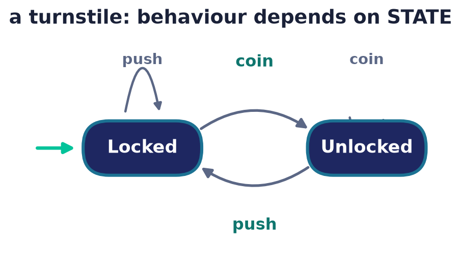
Because the same input can now produce different outputs depending on the stored state, sequential circuits can count, remember, detect patterns over time, and implement protocols — none of which a combinational circuit can do. A pocket calculator’s “+” key does something different depending on what you typed before; a turnstile behaves differently locked versus unlocked; a traffic light cycles. Each needs memory of the past.
The flip-flop stores one bit of state. The atomic memory element of sequential hardware is the flip-flop: a one-bit register that holds a or a between clock ticks and updates on the tick according to its inputs. A circuit with flip-flops has possible stored configurations, i.e. states. This is the physical incarnation of the abstract “state” of an automaton: a finite automaton with states can be realised by a sequential circuit using flip-flops plus combinational logic to compute the next state and the output. Combinational logic (Lecture 5) and sequential logic (this lecture) are therefore not rivals but layers: the combinational part computes the transition function, the flip-flops hold the state between ticks.
Remark (the pivot word is state). The instant a circuit needs to “remember where it is”, it becomes sequential, and the natural mathematical model of “a device that lives in one of finitely many states” is the finite automaton. Automata theory is, in effect, the algebra of sequential behaviour — the abstract theory of what memory-bounded machines can and cannot do.
14.2 Alphabets, strings, and languages
Before we can say what a machine reads or accepts, we need vocabulary for its input. All of it is elementary set theory (Lecture 2) applied to sequences.
Definition (alphabet, string, length). An alphabet is a finite, non-empty set whose elements are called symbols. A string (or word) over is a finite sequence of symbols from . The length of a string is the number of symbols in it. The unique string of length is the empty string, written .
For example, over the strings of length are . Note and, e.g., .
Definition (concatenation). The concatenation of strings and is , of length . Concatenation is associative, and is its identity: . We write for concatenated with itself times, with .
Remark (a monoid, echoing Lecture 3). The set of all strings under concatenation, with identity , is a monoid — an associative operation with a unit. This is the same algebraic pattern you met when composing relations and functions in Lecture 3; there, composition of functions was associative with the identity function as unit. String concatenation is that structure made concrete.
Definition (, , ). is the set of all strings of length exactly . The Kleene star is the set of all finite strings over (including ); excludes .
Substrings, prefixes, and suffixes are defined the obvious way: is a prefix of if for some , a suffix if for some , and a substring if for some .
Definition (language). A language over is any subset .
A language is just a set of strings — possibly finite (), possibly infinite (), possibly empty (), possibly all of . Because languages are sets, the Boolean operations of Lecture 6 apply verbatim: union , intersection , and complement . Two operations are special to strings:
- Concatenation of languages: .
- Kleene star of a language: , where and . Thus is all concatenations of zero or more strings from .
Common pitfall. (the empty string) and (the empty language) are different objects, and both differ from (the language containing only the empty string). Note but , and .
The central question of the chapter can now be phrased crisply: which languages can a finite-memory machine recognise?
14.3 The abstract machine and the idea of state
We first describe a general abstract machine, so that stronger machines appear later as the same picture with more memory. It consists of an input tape holding a string of symbols, a reader (head) positioned over one cell, and a control unit that is always in some internal state. In one step the machine may read the current symbol, inspect and change auxiliary memory, change the control-unit state, possibly write to the tape, and move the reader.
Definition (configuration). A snapshot of an abstract machine at one instant — its configuration — is the triple (current control state, current memory contents, position of the reader). A computation is a sequence of configurations, each obtained from the previous one by a single legal step.
Definition (finite-state machine). A finite-state machine (finite automaton) is the most restricted such machine: it has no auxiliary memory beyond its control state, its reader moves one symbol per step in a single direction (left to right), and its control unit has a finite set of states . Its control may be deterministic (each situation has exactly one next move) or nondeterministic (a situation may permit several).
The deck writes a general finite machine as the seven-tuple
where is the state set, the input alphabet, the output alphabet, the transition (“movement”) function, the output (“exit”) function, the start state, and the set of final states. This form covers machines that produce output (Mealy/Moore, §14.6). When we care only whether a string is accepted — not what is printed — we discard and and obtain the acceptor studied next.
14.4 Deterministic finite automata
Definition (DFA). A deterministic finite automaton is a five-tuple
where
- is a finite set of states;
- is a finite input alphabet;
- is the transition function: given the current state and the symbol just read, it names the unique next state;
- is the start state;
- is the set of accepting (final) states.
The word deterministic means is a total function: for every state and every input symbol there is exactly one next state — no choices, no missing moves. A DFA has no output alphabet; its “answer” is simply whether it halts in an accepting state.
Cross-reference (Lecture 3). The transition function is exactly a function, and — as Lecture 3 established — a function is a special binary relation that is total (defined on every input pair) and single-valued (at most one output). Determinism is nothing more than “ is a genuine function, not merely a relation.” When we drop those two conditions in §14.7 we get exactly the relational — nondeterministic — machine.
Definition (transition table). Because has a small finite domain, we list it completely as a transition table with one row per state and one column per input symbol; the entry is the next state. The start state is marked with an arrow and each accepting state with a star .
Definition (state diagram). The same is drawn as a labelled directed graph (Lecture 10): one node per state, and an edge for each transition . The start state has an incoming arrow “from nowhere”; accepting states are drawn as double circles. Reading a string means walking the graph, following the edge labelled by each symbol in turn.
The extended transition function
tells us what one symbol does. To speak of whole strings we lift it to .
Definition (extended transition function). Define by recursion on the length of the string:
where and .
So is the single state reached after reading all of from . The following bookkeeping lemma — that respects concatenation — is used repeatedly (in the product and subset constructions, and in the pumping lemma), so we prove it once.
Lemma 14.1 (concatenation law for ). For every state and all strings ,
Proof. Fix and ; induct on .
Base , i.e. . Then , so the left side is . The right side is , which equals by the first clause of the definition. The two sides agree.
Inductive step. Suppose the identity holds for a string ; we prove it for with . Using the definition of , then the induction hypothesis, then the definition again:
This is the claim for , completing the induction.
Runs, acceptance, and the language of a DFA
Fix a DFA and an input .
Definition (run). The run of on is the sequence of states with and for . Equivalently . Because is deterministic, each string has exactly one run.
Definition (acceptance and language). accepts if its run ends in an accepting state, ; otherwise rejects . The language recognised by is
Definition (regular language — first form). A language is regular if for some DFA .
Design principle. Building a DFA for a target language means choosing states that record exactly the finite amount of information about the input read so far that is needed to decide acceptance — and no more, since only finitely many states are allowed. Each state is an equivalence class of histories: two input prefixes that must be treated identically from now on may share a state. (This idea, made precise, is the Myhill–Nerode theorem, which we only name here.)
14.5 Worked DFA designs
We now design and verify several DFAs. Each verification is either a full trace or an induction certifying is what we claim.
Example A — even number of $1$s
Task. Over , accept exactly the strings with an even number of $1$s (zero is even, so is accepted).
Design idea. The only fact we must remember is the parity of the count of $1$s. Parity has two values, so two states suffice. Reading leaves parity unchanged; reading flips it.
Formal definition.
| State | on 0 |
on 1 |
|---|---|---|
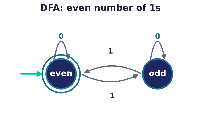
State diagram (in words). Two nodes. is a double circle with the
start arrow into it; is a single circle. Each state has a self-loop
labelled 0. Two arrows labelled 1 cross between the states, one each way.
Trace on 1001 (two $1$s, should accept):
| Step | State before | Symbol | State after |
|---|---|---|---|
| start | — | — | |
| 1 | 1 |
||
| 2 | 0 |
||
| 3 | 0 |
||
| 4 | 1 |
Ends in : accepted. On 1011 (three $1$s) the run is
,
ending outside : rejected. Both correct.
We can do better than spot checks and prove correctness.
Proposition 14.2. For every , if has an even number of $1$s, and otherwise. Consequently , where is the number of $1$s in .
Proof. Induct on . Base: has (even) and . Step: write and assume the claim for . If then and, since for both states, ; the parity and the state both stay put, so the correspondence persists. If then (parity flips) and swaps the two states (state flips); flipping both sides of the induction hypothesis preserves the correspondence. Finally iff iff is even.
Example B — ends in 01
Task. Over , accept the strings that end in 01.
Design idea (suffix matching). Let each state record the longest suffix of the
input read so far that is a prefix of the pattern 01. The prefixes of 01 are
, 0, 01, giving three states: (no useful suffix), (ends in
0), (ends in 01, accepting).
| State | on 0 |
on 1 |
|---|---|---|
Reading the table. From (“…0”) a further 0 still ends in 0 ();
a 1 completes 01 (). From (“…01”) a 0 ends in 0 (); a
1 ends in 11, no useful suffix ().
Traces. 0101: (accept — indeed ends 01). 011:
(reject — ends 11).
Remark (a template). Example B generalises: to accept strings ending in a fixed pattern , use one state per prefix of (the states of the Knuth–Morris–Pratt string matcher). To accept strings containing as a substring, do the same but make the “matched all of ” state absorbing and accepting — see Example C.
Example C — contains the substring 001
Task. Over , accept every string that has 001 somewhere inside.
Design idea. Track progress toward matching 001; once matched, latch into an
accepting sink.
| State | meaning | on 0 |
on 1 |
|---|---|---|---|
| no progress | |||
seen 0 |
|||
seen 00 |
|||
seen 001 (done) |
Two subtle entries. From (“…00”) reading 0 keeps the last two symbols
00, so we stay at (not fall back). From (“…0”) reading 1 gives
suffix 01, which shares no prefix with 001, so we reset to .
Trace on 01001 (contains 001 at positions 3–5): — accept.
Trace on 0100 (no 001): — reject. Correct.
Common pitfall. A frequent bug is sending back to or on
reading 0. But ...000 still ends in 00, so we must stay at ; forgetting
this makes the DFA miss matches like 0001. Always ask: after this symbol, what is
the longest pattern-prefix that is now a suffix of the input?
Example D — binary numbers divisible by
Task. Over , reading a binary numeral most-significant bit first, accept exactly those whose value is divisible by . (Take to denote , which is divisible by .)
Design idea (running remainder). Let the state be the value read so far modulo : states . Appending a bit changes the value to , so the remainder becomes . Compute all six entries:
- : , ;
- : , ;
- : , .
| State | on 0 |
on 1 |
|---|---|---|
Traces. 110 : — accept ().
1001 : — accept ().
101 : — reject (). All correct.
Proposition 14.3. After reading numeral , the DFA of Example D is in state where .
Proof. Induct on . Base : value , state . Step: . By IH the state after is with . Then , so , which is exactly the column the table follows from on . Hence the state after is .
Since , acceptance holds iff , as required. Remark. The same trick — “state = residue of a running quantity” — gives DFAs for divisibility by any fixed modulus and for many counting conditions.
Example E — a “dead state” and totality
Task. Accept strings that begin with 1.
| State | on 0 |
on 1 |
|---|---|---|
Once the first symbol is seen the verdict is fixed, so and are absorbing (all their edges are self-loops).
Common pitfall (totality). A DFA’s must be defined for every
(state, symbol) pair. When a partial design “has no move” for some case — here, a
string starting with 0 should never be accepted — you must add an explicit
dead (trap) state that absorbs all such inputs and is non-accepting. Diagrams
often omit the dead state for readability, but formally it is present. Forgetting it
turns your DFA into an NFA (or into nonsense).
14.6 Machines with output: Mealy and Moore
DFAs answer a yes/no question. Real sequential circuits usually also emit output as they run (think of a controller driving actuators). Adding an output alphabet and an output function to the finite automaton gives a finite-state transducer, and there are two standard flavours, distinguished by where the output lives. (There are no accepting states here: a transducer transforms an input string into an output string.)
Definition (Moore machine). A Moore machine is where output depends only on the current state, . Passing through states on an input of length , it emits — one symbol per state entered, including an initial output before any input, hence output symbols.
Definition (Mealy machine). A Mealy machine has the same shape but its output depends on the current state and the input symbol, so output is attached to transitions: . On an input of length it emits exactly output symbols, one per transition.
Both are captured by the transducer tuple , in which is left unused because a transducer has no accepting states: is the transition function , is the output function , and . The sole difference is whether may read the current input symbol (Mealy) or not (Moore).
Shared example — a running-parity reporter
Reuse the parity machine of Example A, but now report the running parity of $1$s after each symbol instead of only accepting at the end. States (“even so far”) and (“odd so far”); output alphabet (report for even, for odd).
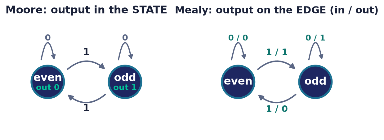
Moore version (output labels the state, ):
| State | output | on 0 |
on 1 |
|---|---|---|---|
0 |
|||
1 |
On input 1011 it visits and prints 01101 (the leading 0 is ’s
output before any symbol is read).
Mealy version (output labels the transition — report the parity after the step):
| State | on 0 (next / out) |
on 1 (next / out) |
|---|---|---|
/ 0 |
/ 1 |
|
/ 1 |
/ 0 |
On the same input 1011 it prints 1101 — the Moore output without the initial
symbol.
What the comparison shows. Moore output is stable while the machine sits in a state (convenient in hardware, where the output is just a function of the flip-flop contents) and carries one extra initial symbol. Mealy output reacts on the same step the input arrives and often needs fewer states. The two are equivalent in power:
Theorem 14.4 (Mealy Moore, informal). For every Moore machine there is a Mealy machine producing the same output (minus the initial symbol) on every input, and vice versa.
Construction sketch. Moore Mealy: set the Mealy output on the transition into a state to that state’s Moore output, i.e. . Mealy Moore: split each state into copies tagged by the output symbol most recently produced, so “which output to emit” becomes a property of the (new) state; the number of states grows by at most a factor of . Both directions are routine inductions on input length, which we omit.
Cross-reference (sequential circuits). A Mealy/Moore machine is the mathematical model of the sequential circuit of §14.1: the flip-flops store the state , one block of combinational logic (Lecture 5) computes the next state from the stored state and the current input, and a second block computes the output . Moore outputs depend on the register only; Mealy outputs also read the current input wire.
14.7 Nondeterministic finite automata
Determinism forces exactly one move per (state, symbol). Relaxing that gives a model that is frequently far easier to design.
Definition (NFA). A nondeterministic finite automaton is a five-tuple where the transition function returns a set of states,
allowing (i) several next states on a symbol, (ii) no next state (the empty set — a dead end), and (iii) -transitions that change state without reading input. Everything else is as for a DFA.
Cross-reference (Lecture 3). Where a DFA’s was a function, an NFA’s is a general relation presented as a set-valued map. This is precisely the loosening — “drop single-valuedness and totality” — foreshadowed in §14.4.
Definition (acceptance for NFAs). accepts if there exists at least one run — one way of resolving the choices, possibly taking -moves — that reads all of and ends in an accepting state. Think of it as existential: the machine accepts iff some computational path succeeds. ( is defined as the set of accepted strings, exactly as before.)
To make “reachable via -moves” precise we need one notion.
Definition (-closure). For a set , the -closure is the set of all states reachable from some state of by following zero or more -transitions. (Formally, the smallest set containing and closed under .)
We can now give the NFA analogue of , this time set-valued:
and accepts iff . (If there are no -moves, is the identity and the formulas simplify.)
Example F — “ends in 01”, the easy way
An NFA can guess where the final 01 begins:
| State | on 0 |
on 1 |
|---|---|---|
State loops on every symbol (staying in “still reading the bulk”); on a 0 it
also forks into , betting that this 0 starts the final 01. From a
1 confirms the bet and reaches accepting ; any other continuation from
or dies. The string is accepted iff some fork survives to the end in ,
i.e. iff the last two symbols are 01.
Remark (why NFAs matter — succinctness). Consider . An NFA needs only states (guess the position, then count more symbols). But any DFA for needs at least states, because it must remember the last symbols — the possible windows are pairwise distinguishable. Nondeterminism buys exponential succinctness, even though — as we now prove — it buys no extra recognising power.
14.8 The subset construction: NFA DFA
The pivotal theorem of the chapter says nondeterminism is a convenience, not a new capability. The construction is the natural one: run the NFA and, at each step, track the set of all states it could currently be in. That set is a single DFA state.
Theorem 14.5 (Rabin–Scott, subset construction). For every NFA there is a DFA with .
Proof. We first treat the case with no -transitions, then note the one change needed for the general case.
Construction. Define by
is a legitimate DFA: is a total single-valued function on (a union of sets is one well-defined set, even when it is empty), and is finite (it has elements). Write for ’s extended transition function.
Key lemma. For every ,
i.e. the DFA state after reading is exactly the set of NFA states reachable on . We prove it by induction on .
Base : by definition of , and (no -moves). Equal.
Step : using the definition of , then the induction hypothesis, then the definition of , then the definition of :
This closes the induction.
Conclusion. Now chase the definitions:
using the key lemma at the third step and the NFA acceptance definition at the last. Hence .
The -case. If has -moves, replace the start state by and the transition rule by — that is, take the -closure after every step. The identical induction (now using the -aware definition of ) gives the same conclusion.
Corollary 14.6. DFAs and NFAs recognise exactly the same class of languages. (Every DFA is trivially an NFA; Theorem 14.5 gives the converse.)
Remark (only reachable subsets matter). Although can be huge, in practice one builds lazily, generating only the subsets actually reached from . Often these are few. This is the standard NFA-to-DFA algorithm inside regex tools.
Worked subset construction
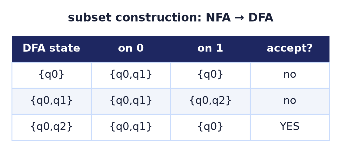
Apply the construction to the NFA of Example F (states , no -moves). Start from and compute reachable subsets:
Only three subsets appear. Rename , , ; accepting subsets are those meeting , namely alone.
| State | on 0 |
on 1 |
|---|---|---|
This is character-for-character the hand-built DFA of Example B. The subset
construction rediscovered our suffix-tracking machine — a satisfying confirmation
that the two designs recognise the same language, “ends in 01”.
Worked subset construction with -moves
Let recognise : states (start), ; , , ; accepting . First the closures: and .
Start (accepting — contains ).
and the empty set is an absorbing non-accepting dead state.
| State | on a |
on b |
|---|---|---|
Traces. aab: accept (). aba:
reject (aba is not of the form ). ba:
reject. All correct.
14.9 Regular expressions and Kleene’s theorem
We have two automaton-based definitions of “regular” (DFA and NFA, now known equal). There is a third, purely syntactic one.
Definition (regular expression). The regular expressions over , and the language each denotes, are defined by recursion:
- is a regex with ;
- is a regex with ;
- each is a regex with ;
- if are regexes, so are , , and , with
Binding tightest to loosest: , then concatenation, then . So means .
For instance denotes “ends in 01”;
denotes “contains 001”; denotes (with for
). These are the same languages we built machines for.
Theorem 14.7 (Kleene, 1956 — stated). A language is regular (recognised by some DFA/NFA) if and only if it is denoted by some regular expression.
We do not give the full two-way proof, but the forward-hard direction is short and ties the chapter together, so we sketch it; the converse is noted.
Regex NFA (Thompson’s construction, sketch). Build an -NFA by recursion on the regex, maintaining the invariant “one start state, one accepting state.” Base cases are one- or two-state machines. For , add a new start with -edges into the two sub-machines’ starts and a new accept with -edges from their accepts. For , glue ’s accept to ’s start with an -edge. For , add a new start/accept state with -edges to ’s start, from ’s accept back to ’s start, and straight through for the empty string. Each rule adds states, so the NFA has size linear in the regex; by the subset construction (Theorem 14.5) it converts to a DFA. This is exactly how regex libraries compile a pattern.
NFA regex (converse, noted). Eliminate states one at a time from the automaton, relabelling the remaining edges with regexes that account for the removed state’s paths (the state-elimination / GNFA method), until a single edge labelled by the answer regex remains.
Definition (regular language — final form). By Corollary 14.6 and Theorem 14.7, the following are the same class of languages, the regular languages: those recognised by a DFA; by an NFA; and those denoted by a regular expression. “Finite automaton”, “regular language”, “regular expression” are three views of one idea — the languages a finite-memory machine can recognise.
14.10 Closure properties of the regular languages
The regular languages are remarkably robust: combine them with the natural set and string operations and you stay regular. These closure theorems are workhorses — both for building machines compositionally and (via §14.11) for proving non-regularity. Note how they mirror the logical connectives of Lecture 6: union is “or”, intersection is “and”, complement is “not”.
Theorem 14.8 (closure under complement). If is regular over , so is .
Proof. Take a DFA with — crucially a DFA, whose is total, so every string has a run ending in a well-defined state. Form by swapping accepting and non-accepting states. Since the run of a string is identical in and , for every ,
Hence .
Common pitfall. This works only for a complete DFA. Swapping the accepting set of an NFA does not complement its language (because “some path accepts” and “some path rejects” can both hold at once). Determinise first, ensure is total, then swap.
Theorem 14.9 (product construction: closure under intersection and union). If are regular, so are and .
Proof. Let be DFAs with . Run both in parallel on one input by taking states to be pairs:
Choose for intersection, or for union.
Parallel-run lemma. for all . Induct on : base gives on both sides; step ,
Now for intersection, iff iff and iff . The union case is identical with “and” replaced by “or”.
Worked use. To accept binary strings with an even number of $0$s AND an odd number of $1$s, take the product of the two 2-state parity DFAs: states , start , accepting the single state .
Theorem 14.10 (closure under union, concatenation, star). If are regular, so are , , and .
Proof (via NFAs). Take NFAs for and use the Thompson gadgets of §14.9. Union: a new start with -edges into both starts. Concatenation: -edges from ’s accepting states to ’s start; start ’s start, accept ’s accepts. Star: a new start/accept state with an -edge to ’s start, -edges from ’s accepts back to its start, and acceptance of built in. In each case one checks the -NFA accepts exactly the intended language; the subset construction then yields a DFA. (These three operations are precisely the constructors of regular expressions — this theorem is the “” of Kleene’s theorem in disguise.)
Corollary 14.11 (closure under set difference). If are regular, so is — a regular language by Theorems 14.8 and 14.9.
Remark (closure as a proof tool). Closure runs backwards too. If we already know some language is not regular, and we can manufacture from a suspect language using operations that preserve regularity, then cannot be regular either — otherwise would be. We exploit exactly this in §14.11.
14.11 The limits of finite memory: the pumping lemma
Everything so far builds regular languages. We now prove that some languages are not regular — that finite memory is a genuine limitation. The tool is the pumping lemma, whose engine is the pigeonhole principle (Lecture 8): a run longer than the number of states must repeat a state, and a repeated state is a loop we can traverse any number of times.
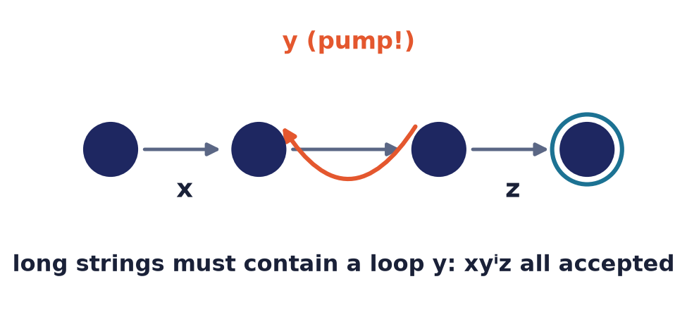
Theorem 14.12 (pumping lemma for regular languages). If is regular, then there is a constant (a pumping length) such that every string with can be split as with
- (the middle part is non-empty),
- (the loop occurs within the first symbols), and
- for all (the middle part may be “pumped”).
Proof. Since is regular, fix a DFA with , and set , the number of states. Let with . Consider the run
Look at the first of these states, . They are states drawn from a set of only states, so by the pigeonhole principle two of them coincide: there exist indices with and .
Define the split
Then (condition 1) and (condition 2). Reading from state returns to , so — a loop. By Lemma 14.1 (concatenation law) and induction on , for every : going around the loop any number of times lands back at . Therefore, again by Lemma 14.1,
Since , we have ; hence , i.e. for all (condition 3).
How to use it (the adversary game). The lemma is a one-directional implication: regular pumpable. To prove a language is not regular we use the contrapositive as a game against an adversary:
- (Adversary) Suppose were regular; it hands you some pumping length (you do not get to choose ).
- (You) Choose a specific string with , cleverly, usually in terms of .
- (Adversary) Splits subject only to and (you must handle every legal split).
- (You) Exhibit one with . That contradicts the lemma, so is not regular.
Worked non-regularity proof:
Theorem 14.13. is not regular.
Proof. Suppose, for contradiction, that is regular, and let be a pumping length from Theorem 14.12. Choose
By the pumping lemma with and . Because the first symbols of are all $0$s, the prefix (of length ) consists solely of $0$s; in particular for some . Pump with :
Since this string has more $0$s than $1$s, so it is not of the form and — contradicting condition 3. Therefore is not regular.
Intuition. demands matching an unbounded count of $0$s against an equal count of $1$s. A finite automaton has only states, so after reading enough $0$s it must reuse a state and thereby “forget” exactly how many it has seen. The pumping lemma turns that forgetting into a concrete counterexample.
A second worked proof: perfect squares of $0$s
Theorem 14.14. (strings of $0$s whose length is a perfect square) is not regular.
Proof. Suppose is regular with pumping length . Choose (note since ). Write with ; say , so . Pump to : the string has length . Now
So lies strictly between the consecutive squares and and is therefore not a perfect square; hence , a contradiction. Thus is not regular.
Remark (pairing with closure — equal $0$s and $1$s). Let . Is regular? Suppose it were. The language is regular (regex ), so by closure under intersection (Theorem 14.9) would be regular. But
which is not regular (Theorem 14.13) — contradiction. Hence is not regular. This is the “closure as a proof tool” remark of §14.10 in action: we avoided a fresh pumping argument by reducing to one we already had.
Common pitfall. (a) You do not choose ; you must survive whatever the adversary picks. (b) You do not choose the split ; you must defeat every split obeying . Choosing (rather than, say, ) is what forces into the -block via . (c) The lemma is not an “if and only if”: some non-regular languages happen to be pumpable, so a successful pump does not prove regularity. Use the lemma only to prove non-regularity.
14.12 Beyond finite automata (a signpost)
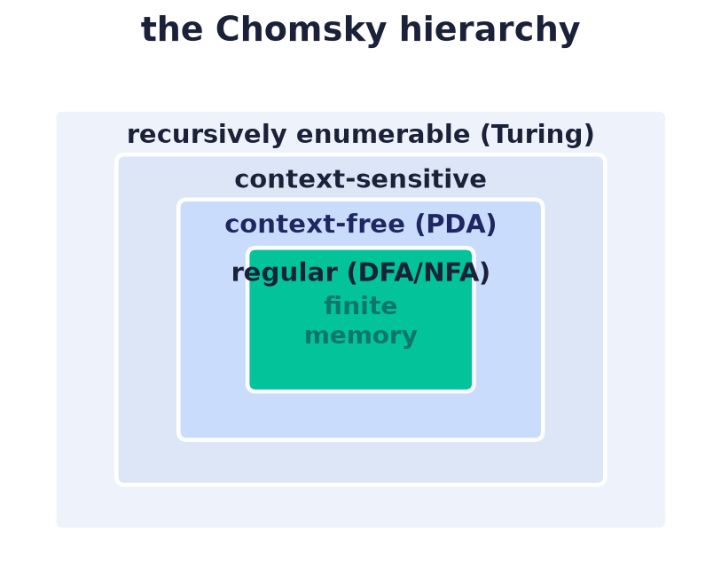
A finite automaton is the weakest standard abstract machine: its only memory is its state. The languages just shown non-regular are not exotic — they are the bread-and-butter of programming languages (balanced brackets, -style matching). To recognise them we must add memory to the same tape-reader-control picture of §14.3:
- Add a stack (last-in-first-out memory) and you get a pushdown automaton, which recognises the context-free languages — enough for , balanced parentheses, and the grammars of programming languages.
- Add an unbounded read/write tape and you get a Turing machine, the most general model of computation, recognising the recursively enumerable languages.
These sit at higher rungs of the Chomsky hierarchy (regular context-free context-sensitive recursively enumerable) and are the subject of a full course in the theory of computation. They lie beyond this introduction; we mention them only to place finite automata on the map. Likewise the DFA-minimisation algorithm (there is a unique smallest DFA per regular language, computable by merging indistinguishable states — the algorithmic face of Myhill–Nerode) is noted but not developed here.
Historical note
The finite-state idea was first written down by Warren McCulloch and Walter Pitts in 1943, who modelled networks of idealised neurons as devices with a finite number of states. Stephen Cole Kleene, analysing those nerve nets in a 1951 RAND memorandum published in the 1956 volume Automata Studies, introduced regular events (our regular expressions) and proved the equivalence now called Kleene’s theorem (Theorem 14.7). The output-producing machines are named for their inventors at Bell Labs: George H. Mealy (“A Method for Synthesizing Sequential Circuits”, 1955) attached output to transitions, while Edward F. Moore (“Gedanken-experiments on Sequential Machines”, 1956) attached it to states. Michael O. Rabin and Dana Scott introduced nondeterministic automata and the subset construction (Theorem 14.5) in their 1959 paper “Finite Automata and Their Decision Problems”, work for which they shared the 1976 Turing Award. The pumping lemma and the algebraic characterisation of regularity (Myhill–Nerode) followed in the late 1950s. It is a striking feature of the subject that a single, small abstraction — the finite automaton — was reached almost simultaneously from neuroscience, logic, and circuit engineering.
CS connections
Finite automata are not a museum piece; they run inside tools you use daily.
- Lexical analysis (lexers). The first phase of every compiler chops source code into tokens (identifiers, numbers, operators). Each token class is described by a regular expression; a tool like lex/flex compiles the union of them (via Thompson’s construction and the subset construction) into a single DFA that scans the source in linear time. This is §14.8–14.9 turned into a product.
- Regular-expression engines.
grep, RE2, and lexer generators simulate an NFA or its determinised DFA. Ken Thompson’s 1968grepused exactly the on-the-fly NFA simulation of §14.7; guaranteed-linear engines (RE2) determinise lazily as in the remark after Theorem 14.5, avoiding the exponential blow-up that “backtracking” regex engines suffer. - Network protocols. TCP connection management is specified as a finite-state
machine (states
LISTEN,SYN-SENT,ESTABLISHED,TIME-WAIT, …); the transitions are triggered by packets and timeouts — a Mealy/Moore machine in production. - Digital hardware. Controllers, vending machines, and traffic lights are synthesised directly from Mealy/Moore descriptions (§14.6) into flip-flops plus combinational logic (§14.1) — closing the loop back to Lecture 5.
- String search and validation. The Knuth–Morris–Pratt matcher is essentially the substring-DFA of Example C; input validation for dates, phone numbers, and URLs is DFA membership testing.
Chapter summary
- Combinational vs sequential. Combinational logic (Lecture 5) computes a fixed Boolean function of the current inputs (adders, decoders, ALU); sequential logic adds state, held in flip-flops ( flip-flops states), so output can depend on the past. State is exactly what automata theory formalises.
- Vocabulary. An alphabet , strings under concatenation (a monoid with unit ), and languages ; distinguish , , and .
- DFA with total ; the extended satisfies the concatenation law (Lemma 14.1); accepts iff , and . Design = pick states recording just-enough finite information (parity, running remainder, suffix progress); always total (add a dead state).
- Mealy vs Moore transducers attach output to transitions vs states; they are interconvertible and model sequential circuits exactly.
- NFA allows set-valued transitions and -moves; it accepts if some path succeeds. The subset construction (Theorem 14.5) determinises any NFA, so DFAs and NFAs recognise the same class — but NFAs can be exponentially smaller.
- Regular languages = DFA-recognisable = NFA-recognisable = regular-expression denotable (Kleene, Theorem 14.7). The class is closed under union, intersection (product construction, Theorem 14.9), complement (swap accepting states of a DFA, Theorem 14.8), concatenation, and Kleene star (Theorem 14.10).
- Pumping lemma (Theorem 14.12): long strings in a regular language contain a pumpable loop. Its contrapositive proves non-regularity: , , and equal-count languages are not regular (Theorems 14.13–14.14) — finite memory has real limits.
- Beyond: adding a stack gives pushdown automata (context-free); an unbounded tape gives Turing machines. Minimisation (Myhill–Nerode) is noted, not developed.
Exercises
Warm-up
1. Let . List all strings of length over , and give , , and the string . Explain why .
2. For the even-number-of-$1$s DFA (Example A), trace the runs on 11010 and on
010, and state whether each is accepted.
3. Write out the five components of the DFA tuple and say how each corresponds to the Mealy/Moore transducer tuple of §14.6 — and which two components a transducer adds.
4. For the “ends in 01” DFA (Example B), trace 1101 and 0010 and give the
verdicts.
5. For the running-parity transducer (§14.6), write the full Moore and
Mealy output strings on input 0110, and explain why they differ in length by
exactly one.
6. Give a regular expression for each: (a) strings over that begin with
1; (b) strings that end in 01; (c) strings that contain 001.
Standard
7. Design a DFA (states, transition table, start, accepting set) over
for strings whose number of $0$s is divisible by . Trace it on 00100.
8. Design a DFA over for “does not contain 11” (no two consecutive
$1$s). Then, using Theorem 14.8, describe how to obtain a DFA for the complement
(“contains 11”).
9. Use the product construction (Theorem 14.9) to build a DFA for “even number
of $0$s and odd number of $1$s”. Give its four states, start, and accepting set,
and trace 0110.
10. Apply the subset construction to the NFA with states , start , accepting , and , , (all other entries ). List the reachable DFA states and give its table. Which familiar language is this?
11. Give a Mealy machine over input , output , that outputs 1
on exactly the step whose input symbol completes an occurrence of the pattern 01
(and 0 otherwise). Trace it on 10011.
12. For the divisible-by- DFA (Example D), trace 1110 and 10010 and give
the values and verdicts. Confirm against ordinary arithmetic.
13. Prove that the class of regular languages is closed under set difference , citing the theorems you use.
Challenge
14. Prove that is not regular. (Hint: pick and pump down.)
15. Prove that the language of binary palindromes is not regular, where is reversed. (Hint: try .)
16. Prove the regular languages are closed under reversal: if is regular then is regular. (Hint: reverse every edge of an NFA for , swap start and accept roles using an -move.)
17. Show that any DFA recognising the -th symbol from the end is
1 needs at least states. (Hint: exhibit length- strings that are
pairwise distinguishable — for each pair, a suffix that one can complete into
and the other cannot — and argue they must reach distinct states.)
18. A DFA has states and accepts at least one string. Prove it accepts a string of length . (Hint: a shortest accepted string cannot repeat a state, by the pumping argument.) Conclude an algorithm to test whether .
19. Prove the pumping lemma’s index bound is tight in the following sense: give a regular language and a string in it for which pumping with (deleting ) leaves the language, illustrating that condition 3 must hold for all , including .
20. Using closure properties only (no direct pumping), prove that is not regular. (Hint: complement, intersect with , and use Theorem 14.13.)
Selected answers & hints
2. 11010: ; ends in — rejected (three $1$s,
odd). 010: ; ends in
— rejected (one , odd).
5. The running parity of $1$s after reading is
. Moore output on 0110 is 00100 (5 symbols: it visits states
and prints their labels ); Mealy output is 0100 (4 symbols:
one per transition, ). Moore emits one symbol per state visited — there
are states for an input of length , including the pre-input output —
while Mealy emits one symbol per transition, exactly . Hence the length
differs by one, and Moore’s string is Mealy’s with the initial 0 prepended.
6. (a) ; (b) ; (c) .
7. States = (number of $0$s) ; reading 1 is a self-loop
on every state, reading 0 cycles ; start and only
accepting state . On 00100: ; ends
— rejected (four $0$s, ).
9. States are pairs (parity of $0$s, parity of $1$s):
;
start ; accepting the single state . On
0110: ;
ends — rejected (two $0$s even, two
$1$s even, so $1$s not odd).
10. Reachable states with the table
, accepting — the language “ends in
01” (identical to Example B), confirming Theorem 14.5.
11. Reuse Example B’s states as a Mealy machine: on every transition
into (namely ) output 1, otherwise 0. On 10011:
transitions — output 00010.
13. . is regular by complement closure (Theorem 14.8), and the intersection of two regular languages is regular by the product construction (Theorem 14.9); hence is regular.
14. Adversary gives . Choose (). Since , lies in the -block, , . Pump down (): . As , the number of ’s is , which is not , so — contradiction.
16. From an NFA for , build : reverse the direction of every transition, make the old accepting states into (nondeterministic) starts — add a fresh start with -edges to each old accept — and make the sole accepting state. A path spelling from to in becomes a path spelling from to in , so ; determinise if a DFA is wanted.
18. Let be a shortest accepted string and suppose . By the pumping lemma with and , but — contradicting minimality. Hence the shortest accepted string has length . Algorithm: test all strings of length (or, better, check by graph reachability whether any accepting state is reachable from ); iff none is accepted.
20. If were regular, so would be its complement, and intersecting the complement with the regular language gives exactly — non-regular by Theorem 14.13. Contradiction, so is not regular.
Further reading
- Michael Sipser, Introduction to the Theory of Computation — Chapter 1 (regular languages, DFAs/NFAs, the subset construction, regular expressions, and the pumping lemma) is the closest match to this chapter.
- John Hopcroft, Rajeev Motwani, and Jeffrey Ullman, Introduction to Automata Theory, Languages, and Computation — a fuller treatment, including minimisation and the Myhill–Nerode theorem.
- Kenneth Rosen, Discrete Mathematics and Its Applications — the chapter on modelling computation gives a gentler, discrete-math-oriented introduction consistent with this course.
Self-check questions
- State precisely the difference between combinational and sequential logic, and explain why a two-bit counter cannot be built from combinational gates alone.
- Give the five components of and define by recursion. Why must be total?
- Prove that the DFA of Example A recognises exactly the even- strings.
- What does the subset construction show, and why does swapping the accepting set of an NFA fail to complement its language?
- State the pumping lemma and use it to prove is not regular.
- Name the three equivalent characterisations of the regular languages, and list the operations under which the class is closed.