Lecture 12. Special graphs
12.0 Overview: why “special” graphs deserve their own chapter
Lecture 10 introduced graphs in the abstract — vertices, edges, degrees, walks, paths, cycles, connectivity, and the handshake identity — and Lecture 11 turned those objects into algorithms: greedy colouring, breadth-first and depth-first search, Dijkstra’s shortest paths, and the minimum-spanning-tree methods of Kruskal and Prim. A general graph, however, is almost featureless: knowing only that “some vertices are joined by some edges” tells us very little, and most interesting questions about arbitrary graphs are computationally hard.
This lecture studies special families of graphs — graphs carrying extra structure. Structure is exactly what turns a shapeless object into a theorem-rich one: the moment we insist that a graph be acyclic, or that its edges alternate between two colour classes, or that every vertex have even degree, a cascade of clean, provable consequences follows, and efficient algorithms become possible.
The centre of gravity is the tree: a connected acyclic graph. Trees are the single most important non-trivial structure in computer science. They organise:
- file systems — a root directory, folders, files, and the unique path
/home/user/notes.txtfrom root to any file; - expression and parse trees — how a compiler represents
(a + b) * cand how a calculator evaluates reverse Polish notation; - search structures — binary search trees, AVL and red–black trees, B-trees, heaps — where the height of the tree is the cost of an operation;
- prefix codes — Huffman coding builds an optimal full binary tree whose leaves are the symbols of an alphabet;
- decision trees, game trees, syntax trees, phylogenetic trees, and the recursion trees we draw to analyse divide-and-conquer algorithms.
We develop trees with full rigour — their several equivalent characterizations, the leaf-counting lemmas, rooted-tree vocabulary, -ary and binary trees, traversals, and spanning trees — and then survey four further families that recur throughout the course: bipartite, regular, Eulerian, and Hamiltonian graphs. Two of the deepest theorems in elementary graph theory live here, and we prove both in full: the characterization of Eulerian graphs by even degrees (Euler, 1736 — the birth of graph theory), and the characterization of bipartite graphs as the graphs with no odd cycle.
Throughout, is a finite undirected graph with vertices and edges, simple (no loops or parallel edges) unless we explicitly allow a multigraph. We lean constantly on the handshake identity of Lecture 10,
and on its corollary that the number of odd-degree vertices is even.
12.1 Trees: intuition and definition
Imagine wiring up computers into one network as cheaply as possible. You need the network connected (every machine can reach every other), and you do not want to pay for redundant cable, so you avoid cycles (a cycle would let you delete a cable and stay connected). The cheapest connected layout is therefore a connected graph with no cycles — a tree. This tension, “connected but with nothing to spare,” is the essence of treeness, and the characterization theorem below makes it precise in four different languages.
Definition (Tree). A tree is a connected undirected graph that contains no cycle. Equivalently, a connected acyclic graph.
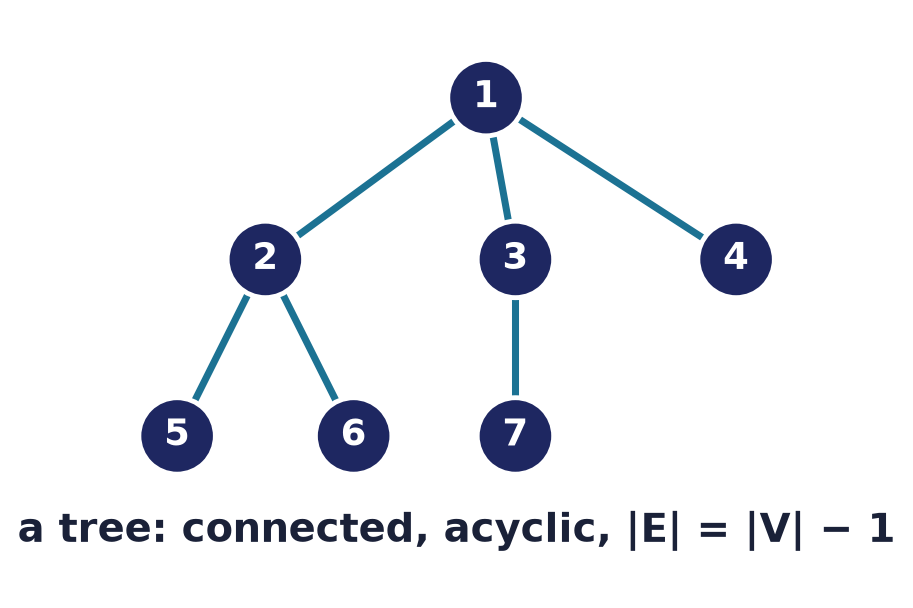
Two words carry the definition. Connected means every pair of vertices is joined by at least one path (Lecture 10). Acyclic means the graph contains no cycle, i.e. no simple closed walk of length (in a simple graph the shortest possible cycle is a triangle). A single vertex with no edges is a tree (vacuously connected and acyclic); so is a single edge.
Remark (why “no cycle of length ”). In a simple graph there are no loops (length-1 closed walks) and no repeated edges (length-2 closed walks), so the smallest possible cycle already has length . When we later allow a multigraph (Königsberg), a pair of parallel edges does count as a cycle of length .
The definitional picture is deceptively simple. What makes trees powerful is that “connected + acyclic” is only one of many equivalent descriptions.
12.2 Leaves and the two-leaf theorem
Definition (Leaf). A leaf (or pendant vertex) of a graph is a vertex of degree . A non-leaf, non-isolated vertex is an internal vertex.
Leaves are the “loose ends” of a tree, and their existence drives almost every proof about trees (they give us something to peel off and induct on). Before the big theorem we isolate the key structural fact.
Theorem 12.1 (Two-leaf theorem). Every tree with vertices has at least two leaves.
Proof. Let be a tree with vertices. Since is finite, among all paths in we may choose one of maximum length; call it
Because is connected and has at least two vertices it has at least one edge, so and the endpoints are distinct. We claim both endpoints are leaves.
Consider . It is adjacent to , so . Suppose, for contradiction, that had another neighbour . There are two cases.
- If does not lie on , then is a path of length , contradicting the maximality of .
- If for some (it cannot be , since ), then is a cycle (its length is ), contradicting that is acyclic.
Both cases are impossible, so has no neighbour other than ; that is, and is a leaf. By the identical argument applied to the other end, is a leaf. Since , the tree has at least two leaves.
Remark. The proof extracts more than the statement: the endpoints of any longest path in a tree are leaves. This “longest path” trick reappears when studying the diameter and centre of a tree.
Common pitfall. The hypothesis is needed. The one-vertex tree has a single vertex of degree — that is not a leaf (leaves have degree exactly ), and the theorem indeed does not claim two leaves there.
12.3 The tree characterization theorem
We first record the exact edge count, then prove the master equivalence. The edge count is proved by peeling off a leaf and inducting — precisely why Theorem 12.1 came first.
Lemma 12.2 (Edge count). A tree with vertices has exactly edges.
Proof. Induction on . Base : the tree is a single vertex with edges. Inductive step: let and assume the claim for all trees with fewer than vertices. By Theorem 12.1, has a leaf with unique neighbour . Form by deleting and its one incident edge .
- is acyclic: deleting a vertex and edges cannot create a cycle.
- is connected: take any two vertices . In there is a path from to . Because , the vertex can appear on a simple path only as an endpoint; since , the – path does not pass through and therefore survives intact in .
Hence is a tree on vertices, so by the inductive hypothesis it has edges. Restoring and the edge adds exactly one edge, so has edges.
Corollary 12.3. In a tree with vertices, . Consequently, if , not every vertex can have degree (that would force the degree sum to be ), re-proving that a tree has at least one — in fact, by Theorem 12.1, at least two — leaves.
We can now state and prove the theorem that makes trees so pleasant to work with.
Theorem 12.4 (Characterization of trees). Let be an undirected graph with vertices. The following are equivalent.
- is a tree (connected and acyclic).
- is connected and has exactly edges.
- is acyclic and has exactly edges.
- Between every pair of vertices there is a unique simple path.
- is minimally connected: connected, but deleting any one edge disconnects it.
- is maximally acyclic: acyclic, but adding any one edge between non-adjacent vertices creates exactly one cycle.
The proof is organised as a cycle establishing the equivalence of the first three, then , , and . We use one small fact repeatedly, stated separately.
Fact 12.5 (Cycle edges are not bridges). If an edge lies on a cycle of a graph , then (delete the edge, keep the vertices) is still connected “through” that pair: any walk using can be rerouted along the rest of the cycle, which is a – path avoiding . Hence removing a cycle edge never disconnects the graph.
Proof of Theorem 12.4.
. Immediate: a tree is connected by definition and has exactly edges by Lemma 12.2.
. Assume is connected with edges; we must show it is acyclic. Suppose not — suppose contains a cycle. By Fact 12.5 we may delete an edge lying on that cycle and remain connected. Repeat: each deletion removes at least one cycle while preserving connectivity. Because is finite this process halts, at a graph that is connected and acyclic, i.e. a tree, on the same vertices. By Lemma 12.2, has edges. But we deleted at least one edge, so has at most edges — a contradiction. Hence was acyclic all along, and being also connected with edges it satisfies (3).
. Assume is acyclic with edges; we must show it is connected. Let have connected components with vertices respectively, where . Each component is connected (by definition of component) and acyclic (a subgraph of an acyclic graph), hence a tree, so by Lemma 12.2 component has edges. Summing,
But by hypothesis, so , giving . Thus has a single component; it is connected, and being also acyclic, it is a tree.
This closes the cycle, so (1), (2), (3) are equivalent.
. Let be a tree. Connectivity gives at least one simple path between any and ; we prove there is at most one. Suppose and were joined by two distinct simple paths and . Reading both from , they begin at the common vertex ; let be the last vertex up to which they agree (so the two paths share the initial segment ending at but take different edges immediately after ). Both paths eventually reach . Follow onward from and let be the first vertex strictly after on that also lies on beyond ; such a exists because qualifies. Now the segment of from to and the segment of from to
- share only their endpoints and (by the minimal choice of , no interior vertex of the -segment lies on beyond ), and
- differ in their first edge out of (by the choice of ),
so together they form a closed walk that repeats no vertex except at the ends — a cycle. (Its length is : the two – segments are distinct and, in a simple graph, at most one of them can be the single edge , so their total length is at least .) This contradicts acyclicity. Hence the path is unique.
. Suppose every pair of vertices is joined by a unique simple path. Existence of a path for every pair means is connected. And is acyclic: a cycle through two of its vertices would provide two distinct – paths (its two arcs), contradicting uniqueness. So is a tree, and .
. Let be a tree; it is connected. Take any edge . By the only simple – path is the single edge itself. Removing therefore leaves no – path (a surviving path plus would be a cycle, impossible), so is disconnected. Thus is minimally connected.
. Suppose is minimally connected. It is connected by hypothesis. If it had a cycle, Fact 12.5 lets us delete a cycle edge and stay connected, contradicting minimality. So is acyclic — a tree. Hence .
. Let be a tree; it is acyclic. Let be non-adjacent, and add the edge . By there is a unique simple – path in ; then is a cycle. It is the only cycle in : every cycle of must use (since itself is acyclic), and a cycle through consists of together with a simple – path in — of which there is exactly one. So adding creates exactly one cycle; is maximally acyclic.
. Suppose is maximally acyclic; it is acyclic. If were disconnected, pick in different components. They are non-adjacent, and adding creates no cycle (a cycle would require a pre-existing – path, but they lie in different components). That contradicts maximal acyclicity, which demands that adding an edge create a cycle. So is connected — a tree, and .
All six statements are equivalent.
Worked example. Take vertices with edges .
        2
        |
        1
        |
        3
       / \
      4   5
          |
          6
There are vertices and edges; the graph is connected and has no cycle, so it is a tree (any one of characterizations (1)–(3) certifies this). The unique path from to is , illustrating (4). Deleting the edge splits it into and , confirming minimal connectivity (5). The leaves are (degree ); vertex has degree . Degree sum , matching Corollary 12.3.
Common pitfall (the count is not by itself sufficient). Having edges does not make a graph a tree. The 4-vertex graph consisting of a triangle plus an isolated vertex has and , yet it is neither connected nor acyclic. Characterization (2) requires both edges and connectivity; (3) requires both edges and acyclicity. Drop either extra hypothesis and the statement fails.
12.4 Forests
Definition (Forest). A forest is an acyclic undirected graph (not necessarily connected). Equivalently, a disjoint union of trees: each connected component of a forest is a tree.
Proposition 12.6. A forest with vertices and connected components has exactly edges.
Proof. Let the components be trees on vertices with . By Lemma 12.2 component has edges, so the total is .
A tree is the special case , recovering . Turning the equation around, : in a forest, the number of components equals vertices minus edges. This is the tiny counting engine behind the union–find data structure used by Kruskal’s MST algorithm (Lecture 11): each accepted edge merges two trees into one, dropping the component count by exactly one.
Example. A graph on vertices made of one -vertex tree, one -vertex tree, and one isolated vertex is a forest with components; it has edges. Adding an edge that joins two different components lowers to and keeps it a forest; adding an edge inside a single component would create a cycle (by the maximal-acyclic property, Theorem 12.4(6)).
12.5 Rooted trees and terminology
Un-rooted trees are symmetric — no vertex is special. Computing almost always wants a distinguished starting point, so we single one out.
Definition (Rooted tree). A rooted tree is a tree in which one vertex is designated the root . Choosing a root orients every edge conceptually away from and imposes a parent–child hierarchy determined by the unique paths of Theorem 12.4(4).
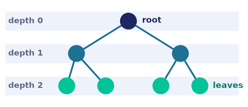
Fix a rooted tree with root . For a vertex :
- Parent — the vertex adjacent to on the unique path from to ; the root has no parent, every other vertex has exactly one.
- Child — any vertex whose parent is .
- Siblings — vertices sharing the same parent.
- Ancestors — the vertices on the path from up to , excluding ; descendants — the reverse relation (’s descendants are the vertices having as an ancestor).
- Leaf — a vertex with no children; internal vertex — a vertex with at least one child. (In a rooted tree “leaf” means childless, which coincides with degree for all non-root vertices, and can also apply to the root if it has a single child in the un-rooted sense — a mild abuse we tolerate.)
- Subtree rooted at — together with all its descendants and the edges among them; itself a rooted tree with root .
- Depth (level) of — the length (number of edges) of the path from to ; the root has depth .
- Height of the tree — the maximum depth over all vertices, i.e. the length of the longest root-to-leaf path.
Depth 0:            A            (root)
                   / \
Depth 1:          B   C
                 / \
Depth 2:        D   E
Example. In the rooted tree drawn above (root ; children of ; children of ): is the root at depth ; are at depth and are siblings; at depth are siblings and children of ; is an ancestor of , and is a descendant of . Leaves are ; internal vertices are . The subtree rooted at is . The height of the tree is .
CS connection (file systems). A Unix-like file system is a rooted tree: the
root directory / is , directories are internal vertices, files are leaves, and
the unique path guaranteed by Theorem 12.4(4) is exactly the absolute pathname
/home/user/notes.txt. Path uniqueness is what makes a pathname a well-defined
address. (Symbolic links deliberately break the tree structure, turning it into a
general graph — which is why link loops can hang naïve directory traversals.)
12.6 -ary and binary trees; counting and height bounds
Definition. An -ary tree is a rooted tree in which every internal vertex has at most children. It is a full -ary tree if every internal vertex has exactly children. A binary tree is the case , with each child distinguished as the left child or the right child — so a binary tree is an ordered rooted tree, and the empty left/right slot matters.
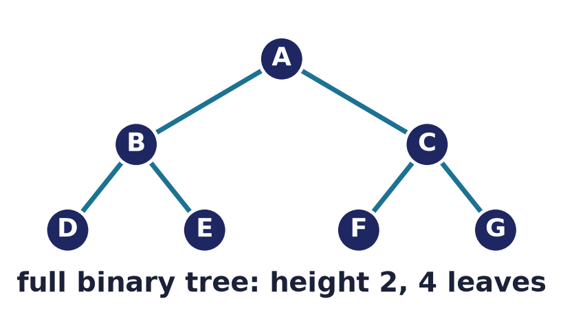
Two further shape adjectives (terminology varies between textbooks, so we pin them down):
- Perfect (a.k.a. complete) -ary tree — full, and all leaves at the same depth.
- Balanced tree — every leaf is at depth or , where is the height; the tree is “as short as possible” for its number of leaves. AVL trees and red–black trees are binary search trees that self-balance after each insertion or deletion, keeping the height .
Counting vertices and leaves in a full -ary tree
Theorem 12.7. A full -ary tree with internal vertices has
Proof. Every vertex except the root is the child of exactly one internal vertex, and each of the internal vertices has exactly children (fullness). Counting children, the number of non-root vertices is ; adding the root gives . The leaves are the vertices that are not internal, so .
For a full binary tree () this reads and : the number of leaves is exactly one more than the number of internal vertices.
Example. A full binary tree with internal vertices has leaves and vertices; check .
CS connection (Huffman coding). An optimal binary prefix code corresponds to a full binary tree: the symbols sit at the leaves, and the codeword for a symbol is the sequence of left/right (0/1) turns from the root. “Prefix-free” means no codeword is a prefix of another, which holds precisely because no leaf is an ancestor of another leaf. Huffman’s greedy algorithm repeatedly merges the two least-frequent subtrees, and guarantees the arithmetic of the merge tree works out.
The height–leaf bound
Theorem 12.8 (Leaf bound). An -ary tree of height has at most leaves.
Proof. Strong induction on . Base : the tree is a single vertex (the root), which is a leaf, so it has leaf. Step: let . The root has at most children; deleting the root splits the tree into at most subtrees, each of height at most , hence each with at most leaves by the inductive hypothesis. Since the root is internal, so every leaf of the whole tree is a leaf of one of these subtrees. Therefore the number of leaves is at most .
Corollary 12.9 (Height lower bound). An -ary tree with leaves has height . For binary trees, .
Proof. From take base- logarithms: . As is an integer, .
Counting vertices level by level (at most vertices at depth , proved by the same induction) gives the companion bound: an -ary tree of height has at most vertices, and for binary trees at most .
Example (perfect binary tree). A perfect binary tree of height has levels with vertices, so leaves and vertices in total — the bounds are met with equality exactly for perfect trees.
Example (why balance matters). A binary search tree holding keys in its leaves needs height at least . A balanced tree achieves height , so a lookup touches about nodes; a degenerate tree (a path — every internal node has one child) has height , so a lookup can touch a million nodes. Balancing is exactly the discipline of keeping the height near its lower bound , which is why AVL/red–black trees guarantee operations.
Remark (counting shapes — Catalan numbers). The number of distinct shapes of a binary tree with nodes (left/right distinguished, unlabelled) is the -th Catalan number
so . Catalan numbers also count balanced parenthesizations and full binary trees with leaves — a recurring motif in combinatorics, though beyond our present scope.
12.7 Tree traversals
Definition (Traversal). A traversal of a rooted tree is a systematic order that visits every vertex exactly once. The cost of any of the traversals below is time (each vertex and edge is handled a constant number of times).
We use the specific binary tree of the slides.
(Figure — the slide binary tree.) Root ; ’s children are (left) and (right); ’s children are (left) and (right); ’s children are (left) and (right) — a perfect binary tree of three levels.
          A
        /   \
       B     C
      / \   / \
     D   E F   G
Levels are — depth : ; depth : ; depth : .
Breadth-first (level-order) traversal
Visit vertices level by level, left to right, using a queue: enqueue the root; repeatedly dequeue a vertex, visit it, and enqueue its children left-to-right. For the figure:
This is exactly breadth-first search from the root (Lecture 11) applied to the tree.
Depth-first orders
The three depth-first orders are defined recursively. For a node with left subtree and right subtree :
- Pre-order — visit , then , then (root first).
- In-order — visit , then , then (root in the middle; meaningful for binary trees).
- Post-order — visit , then , then (root last).
Tracing the recursion on the figure:
| Order | Sequence |
|---|---|
| Pre-order | |
| In-order | |
| Post-order |
As a sanity check: the root appears first in pre-order and last in post-order — a property that holds for every rooted tree and is a handy way to spot a miscomputed sequence.
Reconstruction. Pre-order together with in-order (or post-order together with in-order) uniquely determines a binary tree: the pre-order tells you the root; the in-order then tells you which vertices fall in the left subtree (those before the root) and which in the right (those after), and you recurse. This is precisely how the tree above is recovered from the slide’s sequences, and it is a standard exercise and interview question.
Common pitfall. In-order is only well-defined for binary (more generally, ordered) trees, because it must interleave the node “between” its left and right subtrees. For a general -ary or unordered tree, pre- and post-order still make sense but in-order does not.
CS connection (expression trees). An arithmetic expression tree for has at the root, left subtree , and right leaf :
        ×
       / \
      +   c
     / \
    a   b
- Pre-order yields prefix / Polish notation: .
- Post-order yields postfix / reverse Polish notation: .
- In-order (with parentheses) yields the usual infix form: .
Post-order matches a stack machine: scanning , push operands, and on each operator pop its arguments, compute, push the result. This is why reverse Polish calculators and many virtual machines (e.g. the JVM’s operand stack) evaluate in post-order.
12.8 Spanning trees, Cayley’s formula, and the Matrix-Tree theorem
Definition (Spanning tree). Given a connected graph , a spanning tree is a subgraph that (i) is a tree and (ii) contains every vertex of . By Theorem 12.4, a spanning tree has all vertices and exactly edges; it is a minimally connected / maximally acyclic skeleton of .
Theorem 12.10. Every connected graph has a spanning tree.
Proof. Two constructions, either suffices.
Edge-deletion (top-down). While contains a cycle, delete an edge on that cycle. By Fact 12.5 connectivity is preserved and the process strictly decreases the edge count, so it terminates. The result is connected and acyclic — a spanning tree (it still contains every vertex, since we never delete vertices).
Search-tree (bottom-up). Run BFS or DFS from any vertex (Lecture 11). The tree edges — those that first discover a new vertex — form a connected, acyclic, spanning subgraph, hence a spanning tree.
A disconnected graph has no spanning tree, but each component has one; together they form a spanning forest. When carries edge weights, a minimum spanning tree (MST) is a spanning tree of least total weight — constructed by Kruskal’s and Prim’s algorithms in Lecture 11, which we do not repeat here. Spanning trees model loop-free broadcast in networks (the spanning-tree protocol in Ethernet switching exists precisely to break cycles that would otherwise cause broadcast storms).
Counting spanning trees: Cayley’s formula
Theorem 12.11 (Cayley’s formula, 1889). The complete graph has exactly spanning trees. Equivalently, there are distinct labelled trees on the vertex set .
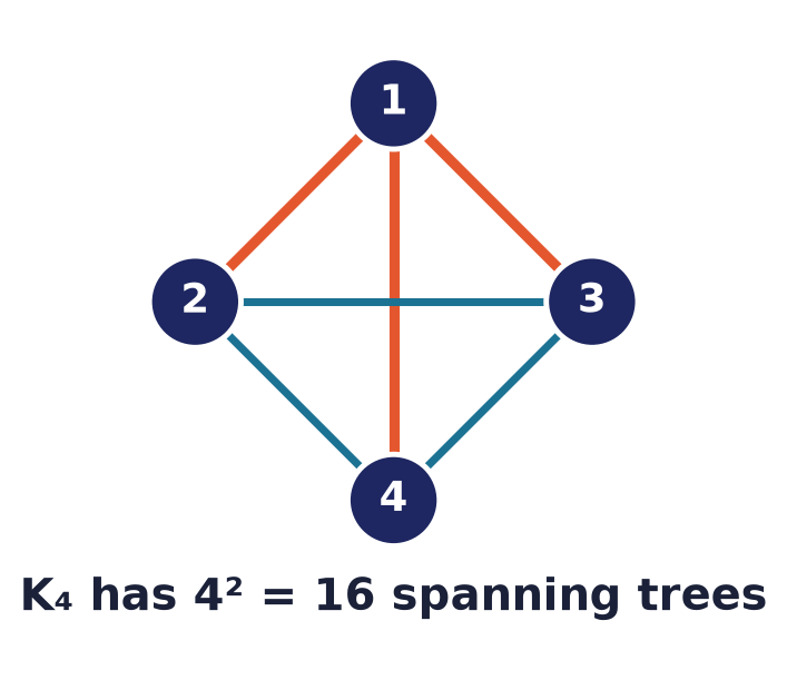
We state it and illustrate it for small rather than proving it in full; the cleanest proof is the bijection of the next paragraph.
- : tree (the single vertex), by convention.
- : tree (the single edge ).
- : trees. Every tree on vertices is a path; the three labelled paths differ by which vertex is the middle: , , .
- : trees. Every tree on vertices is either a path or a star . Labelled paths: (order the four vertices, divide by the two directions). Labelled stars: (choose the centre). Total .
Prüfer’s bijection (idea). Cayley’s exponent is explained by a beautiful encoding due to Prüfer (1918). Given a labelled tree on with , repeat times: find the leaf with the smallest label, record the label of its unique neighbour, and delete the leaf. This produces a Prüfer sequence — a string of length over the alphabet . The map is a bijection between labelled trees and such strings, and there are exactly strings, which is Cayley’s formula. (Decoding reverses the process.) The vertices appearing in the sequence are the internal vertices; a vertex’s number of appearances is its degree minus one — a useful fact in itself.
The Matrix-Tree theorem (for general graphs)
For a graph other than , the count is given by a determinant.
Theorem 12.12 (Kirchhoff’s Matrix-Tree theorem, 1847). Let be a connected graph with adjacency matrix and diagonal degree matrix , and form the Laplacian . Then the number of spanning trees of equals the value of any cofactor of (delete any one row and the matching column, and take the determinant of what remains).
We use it as a black box. Applied to (whose Laplacian is ) it recovers Cayley’s , tying the two results together.
Examples.
- has spanning trees; has ; has .
- The cycle has exactly spanning trees: deleting any one of its edges leaves a path (a tree), and no other subgraph on edges spans it, so there are precisely choices.
K4 (left) and two of its 16 spanning trees:

   1---2        1---2        1   2
   |\ /|        |            |   |
   | X |        |            |   |
   |/ \|        |            |   |
   4---3        4---3        4---3
12.9 Bipartite graphs and the odd-cycle theorem
Definition (Bipartite graph). A graph is bipartite if its vertex set can be partitioned into two disjoint sets (the parts) so that every edge joins a vertex of to a vertex of — no edge has both endpoints in the same part. Equivalently, is properly -colourable: colour red and blue and no edge is monochromatic.
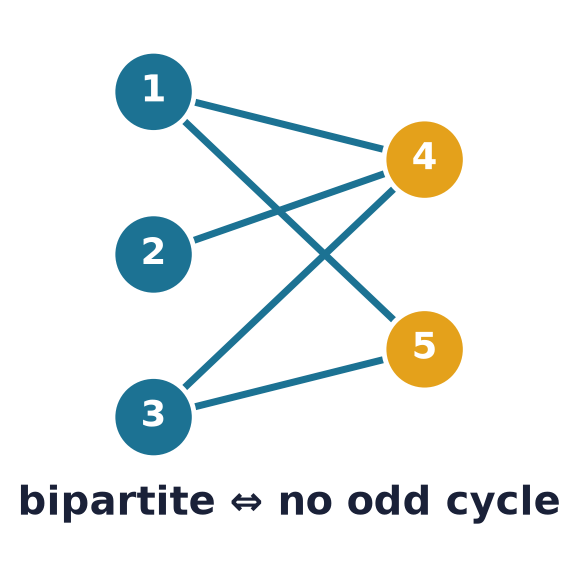
Definition (Complete bipartite graph). has parts of sizes and with every cross pair joined; it has edges.
Bipartite graphs model any two-sided relationship: students–courses, jobs–applicants, tasks–time-slots, senders–receivers. The central question “can these two sides be matched up?” (bipartite matching) is efficiently solvable, whereas the analogous question in general graphs is much harder — another example of structure buying tractability.
Matchings and Hall’s theorem. A matching is a set of edges no two of which share an endpoint; it is perfect if it covers every vertex. In a bipartite graph with parts , whether can be completely matched into is settled by Hall’s marriage theorem: a matching saturating exists if and only if every subset satisfies — no vertices on the left collectively see fewer than neighbours on the right. Necessity is immediate; sufficiency is proved with augmenting paths — find a path that alternates unmatched and matched edges between two exposed vertices and flip it, enlarging the matching until Hall’s condition finally blocks growth. This augmenting-path idea is the efficient algorithm alluded to above.
Theorem 12.13 (Odd-cycle characterization; cf. Lecture 10, Theorem 10.17). A graph is bipartite if and only if it contains no cycle of odd length.
Proof.
() Bipartite no odd cycle. Suppose is bipartite with parts and , and let be any cycle. Each edge crosses between the parts, so the vertices alternate: if then , , and in general iff is even. Returning to forces to be even. Hence every cycle has even length; there is no odd cycle.
() No odd cycle bipartite. It suffices to -colour each connected component, since a disjoint union of bipartite graphs is bipartite (colour the components independently). So assume is connected and has no odd cycle.
By Theorem 12.10, has a spanning tree ; root it at any vertex . Colour each vertex by the parity of its depth in (the length of the unique – path in ): white if even, black if odd. This partitions into two parts; we must check that every edge of joins different colours.
Take an edge .
- If : the depths of and differ by exactly , so their parities differ and the colours differ.
- If : adding to creates exactly one cycle (Theorem 12.4(6)), namely the unique tree path from to together with the edge . This cycle lies in , so by hypothesis its length is even, whence is odd. The tree-path length satisfies
(because , where lca denotes their lowest common ancestor, and is even). Since is odd, and have different parities, so and get different colours.
Every edge is thus bichromatic, so the colouring is proper and is bipartite.
Corollary 12.14. Every tree is bipartite (it has no cycle at all, hence no odd cycle). More generally, every forest is bipartite.
Example. The -cycle is bipartite with parts and : BFS from assigns levels , two colours with no clash. The -cycle is not bipartite — it is itself an odd cycle, so any attempt to -colour it collides after going once around.
Example (the hypercube). The -dimensional hypercube , whose vertices are the binary strings of length with edges between strings differing in one bit, is bipartite: colour each vertex by the parity of its number of $1$s. Every edge flips one bit, hence changes the parity, so it is bichromatic. (This is Exercise S7.)
Common pitfall (Eulerian bipartite, etc.). “Bipartite” constrains cycles (their lengths), while “Eulerian” constrains degrees (their parities). They are unrelated: is both; is both; is Eulerian but not bipartite; the path is bipartite but not Eulerian. Do not conflate a parity condition on cycle lengths with a parity condition on vertex degrees.
12.10 Regular graphs
Definition (Regular graph). A graph is -regular if every vertex has the same degree . A -regular graph is also called cubic.
Proposition 12.15. A -regular graph on vertices has edges. In particular must be even: no -regular graph exists when both and are odd.
Proof. By the handshake identity, , so . Since is an integer, is even.
Familiar regular graphs: the cycle is -regular; the complete graph is -regular; the complete bipartite is -regular; the hypercube is -regular; the Petersen graph is cubic (-regular) on vertices.
Example. Can a -regular graph have vertices? Then is odd, so is not an integer — impossible. A cubic graph must have an even number of vertices (e.g. is cubic on vertices with edges).
12.11 Eulerian graphs and Euler’s theorem
Definition. An Euler circuit (Eulerian circuit) is a closed walk that uses every edge exactly once and returns to its start. An Euler trail (Eulerian path) uses every edge exactly once but may start and end at different vertices. A graph with an Euler circuit is an Eulerian graph.
These conditions are about covering all edges, in contrast to the Hamiltonian conditions of §12.12 which cover all vertices. We prove Euler’s characterization for connected graphs; it holds verbatim for connected multigraphs, which we need for Königsberg. (Isolated vertices, having degree , are irrelevant and are ignored; “connected” means the edges live in one piece.)
Theorem 12.16 (Euler, 1736). Let be a connected (multi)graph with at least one edge.
- has an Euler circuit if and only if every vertex has even degree.
- has an Euler trail but no Euler circuit if and only if exactly two vertices have odd degree; those two are the endpoints of every such trail.
Proof of (1).
() Necessity. Suppose has an Euler circuit . Fix a vertex and walk along . Every time passes through it arrives on one edge and departs on another, consuming two edges incident to ; and because is closed, even the visits at the start/end pair up (the very first edge leaving the start and the very last edge returning to it form one such pair). Since uses each edge exactly once, the edges at are partitioned into these entry–exit pairs. Hence is even, for every .
() Sufficiency. Suppose is connected, has an edge, and every vertex has even degree. We construct an Euler circuit (this is Hierholzer’s algorithm, 1873).
Step 1 — any maximal trail from a vertex is closed. Start at any vertex that has an incident edge and greedily extend a trail (a walk with no repeated edge), leaving each vertex on a not-yet-used edge, continuing as long as possible. Claim: the trail can only get stuck back at . Indeed, consider the moment the trail arrives at some vertex . Counting edges of used so far: each earlier visit to used two (in and out), and this arrival uses one more, an odd total. Since is even, at least one edge at remains unused, so the trail can leave — it is not stuck. Only at can the parity work out to leave no exit. Therefore the maximal trail is a closed trail ending at .
Step 2 — splice in the leftover edges. If uses every edge of , it is an Euler circuit and we are done. Otherwise, let be the subgraph of unused edges. In passing from to we removed the closed trail , which uses an even number of edges at every vertex (entry–exit pairs again), so every vertex of still has even degree. Because is connected, some vertex lying on is incident to an unused edge, i.e. . Apply Step 1 inside starting at to obtain a closed trail through using only unused edges. Now splice into : traverse until reaching , detour completely around (returning to ), then finish . The result is a longer closed trail using strictly more edges.
Step 3 — terminate. Each splice increases the number of used edges, and has finitely many edges, so after finitely many splices every edge is used. The final closed trail is an Euler circuit.
Proof of (2). First, the number of odd-degree vertices is always even (handshake corollary), so “exactly one odd vertex” is impossible and the only traversable cases are or odd vertices.
() Suppose exactly two vertices have odd degree. Add a new edge (a parallel edge if are already adjacent; the graph is allowed to be a multigraph). This raises and by , making all degrees even, and keeps the graph connected. By part (1) there is an Euler circuit; deleting the added edge from it breaks the circuit open into a trail that uses every original edge exactly once and runs between and — an Euler trail.
() Suppose has an Euler trail from to (, since there is no Euler circuit). Add the edge ; the trail plus is an Euler circuit, so by part (1) all degrees in are even. Removing lowers only and by , making exactly and odd and all others even. Thus exactly two vertices () have odd degree, and they are the trail’s endpoints.
Example (Seven Bridges of Königsberg). Königsberg’s four land masses and seven bridges form a multigraph with vertex degrees — four odd-degree vertices.
        (A) 3
        /|  \
       / |   \
    (B)3-+---(C)3        [seven edges = seven bridges]
       \ |   /
        \|  /
        (D) 5
Euler’s theorem needs odd vertices for a circuit or exactly for a trail; with four odd vertices Königsberg has neither — no walk crosses every bridge exactly once. Euler’s 1736 analysis of this puzzle is regarded as the founding result of graph theory. By contrast, is -regular (all degrees even) and connected, so it is Eulerian.
CS connection. The “even degree” condition powers de Bruijn graph genome assembly, where reconstructing a DNA sequence from overlapping fragments reduces to finding an Euler trail. The route-inspection (“Chinese Postman”) problem asks for the shortest closed walk covering every edge and starts from exactly this theory.
12.12 Hamiltonian graphs; Dirac’s and Ore’s conditions
Definition. A Hamiltonian path visits every vertex exactly once. A Hamiltonian cycle (circuit) does so and returns to its start. A graph with a Hamiltonian cycle is a Hamiltonian graph.
Superficially this is Euler’s problem with “edge” replaced by “vertex,” but it is fundamentally harder. There is no known simple necessary-and-sufficient criterion for Hamiltonicity, and deciding whether a graph is Hamiltonian is NP-complete — one of Karp’s original 21 NP-complete problems, and the pure form of the Travelling Salesman Problem. What we do have are useful sufficient (not necessary) conditions that guarantee Hamiltonicity when the graph is “dense enough.”
Theorem 12.17 (Ore, 1960). Let be a simple graph with vertices such that for every pair of non-adjacent vertices . Then is Hamiltonian.
Corollary 12.18 (Dirac, 1952). If is a simple graph with vertices and for every vertex , then is Hamiltonian.
Dirac follows instantly from Ore (any two vertices, adjacent or not, have degree sum ), so we prove Ore. The argument is a classic and illustrates the “maximal counterexample + rotation” technique.
Proof of Theorem 12.17 (Ore). Suppose, for contradiction, that some graph satisfies Ore’s condition yet is not Hamiltonian. Adding an edge never decreases any degree, so Ore’s condition is preserved under adding edges; also, is Hamiltonian for . Therefore, starting from our graph and adding edges one at a time, we reach a graph that is a maximal non-Hamiltonian graph satisfying Ore’s condition: is not Hamiltonian, but adding any missing edge creates a Hamiltonian cycle.
Since is not complete, choose non-adjacent vertices . Adding produces a Hamiltonian cycle, which must use the new edge (it is the only new edge). Deleting from that cycle leaves a Hamiltonian path in from to :
listing all vertices.
Define two index sets inside :
Here (each neighbour of contributes the index ) and (each neighbour of contributes ).
Claim: and are disjoint. Suppose some , so and . Then
is a cycle: (), the middle is the path reversed, and (). It visits every vertex exactly once — a Hamiltonian cycle in , contradicting that is non-Hamiltonian. So .
Both and are subsets of the -element set and are disjoint, so
contradicting Ore’s condition for the non-adjacent pair . This contradiction proves the theorem.
Common pitfall (sufficient, not necessary). Dirac’s and Ore’s conditions can fail on graphs that are Hamiltonian. The cycle (for large ) is Hamiltonian by definition, yet every vertex has degree , so Dirac’s hypothesis fails badly. Never conclude “not Hamiltonian” from the failure of Dirac/Ore.
Necessary conditions (easy direction). A Hamiltonian graph is connected and has minimum degree (a Hamiltonian cycle enters and leaves every vertex). Hence no tree with vertices is Hamiltonian — trees have leaves. Deleting any vertices from a Hamiltonian graph leaves at most components (toughness); this rules out many graphs but is still far from sufficient.
Example. () is Hamiltonian — list the vertices in any order and close the loop; Dirac holds since . Every cycle is trivially Hamiltonian. But the Petersen graph (cubic, vertices) has a Hamiltonian path yet no Hamiltonian cycle — a famous demonstration that regularity and high symmetry are not enough.
12.13 Euler versus Hamilton: a side-by-side
| Eulerian | Hamiltonian | |
|---|---|---|
| Covers every… | edge once | vertex once |
| Clean criterion? | Yes — even degrees (Thm 12.16) | No — NP-complete in general |
| Testable in poly time? | Yes () | Not known (NP-complete) |
| Sufficient conditions | the degree parity is the criterion | Dirac, Ore (dense graphs) |
| Historical seed | Königsberg bridges, Euler 1736 | Icosian game, Hamilton 1857 |
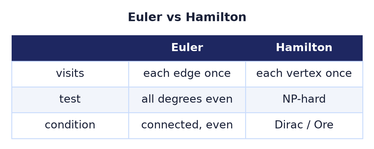
The two properties are independent. The bowtie graph — two triangles sharing a single vertex — is Eulerian but not Hamiltonian: every degree is even (the shared vertex has degree , the rest degree ), yet the shared vertex is a cut-vertex, so no cycle can visit all five vertices exactly once. Conversely, is Hamiltonian but not Eulerian: it contains the -cycle , but all of its degrees are (odd). And is neither. The lesson: an edge condition and a vertex condition genuinely capture different structure.
Common pitfall. Do not assume a graph that “obviously can be drawn in one stroke” is Hamiltonian, or vice versa. Drawing in one pen-stroke is the Eulerian question (traverse each edge/line once); visiting each junction once is the Hamiltonian one.
Historical notes
- 1736 — Leonhard Euler, Solutio problematis ad geometriam situs pertinentis, solved the Seven Bridges of Königsberg, proving no such walk exists and inventing what we now call graph theory. His degree-parity insight is Theorem 12.16.
- 1847 — Gustav Kirchhoff derived the Matrix-Tree theorem (Theorem 12.12) from the theory of electrical circuits, counting spanning trees via determinants.
- 1857 — William Rowan Hamilton marketed the Icosian Game, a puzzle of finding a cycle through all vertices of a dodecahedron — the origin of the term Hamiltonian cycle (though such cycles had been studied earlier by Kirkman).
- 1873 — Carl Hierholzer gave the constructive proof of Euler’s theorem used in §12.11.
- 1889 — Arthur Cayley published the formula for labelled trees (Theorem 12.11); Heinz Prüfer (1918) later gave the elegant bijective proof.
- 1952 — Gabriel Dirac and 1960 — Øystein Ore proved the sufficient degree conditions for Hamiltonicity (Theorem 12.17, Corollary 12.18).
Chapter summary
- A tree is a connected acyclic graph. Theorem 12.4 shows this is equivalent to: connected with edges; acyclic with edges; a unique path between every pair; minimally connected; maximally acyclic. Neither “ edges” alone nor “connected” alone suffices — you need a pair.
- A tree on vertices has exactly edges (Lemma 12.2) and, for , at least two leaves (Theorem 12.1, via the longest-path argument). A forest with components has edges.
- A rooted tree adds root/parent/child/sibling/ancestor/descendant structure, with the depth of a vertex and the height of the tree.
- -ary / binary trees. A full -ary tree with internal vertices has vertices and leaves (Theorem 12.7). Height forces at most leaves (Theorem 12.8), so a tree with leaves has — the reason balanced search trees run in .
- Traversals. Breadth-first (level order) and the depth-first pre-/in-/post-order. On the slide tree: BFS , pre , in , post . Pre+in (or post+in) rebuild a binary tree; expression trees give prefix/infix/postfix notation.
- Spanning trees have all vertices and edges; every connected graph has one. has of them (Cayley, via Prüfer sequences); the Matrix-Tree theorem counts them for any graph.
- A graph is bipartite it is -colourable it has no odd cycle (Theorem 12.13, proved via a spanning tree). Every tree/forest is bipartite.
- A -regular graph on vertices has edges, so is even.
- Euler (Theorem 12.16): a connected graph has an Euler circuit all degrees even; an Euler trail (and no circuit) exactly two odd vertices.
- Hamilton: visits every vertex once; no simple criterion (NP-complete), but Ore ( for non-adjacent ) and its corollary Dirac () are sufficient. Euler is about edges, Hamilton about vertices.
Exercises
Warm-up
W1. Draw all unlabelled trees on vertices, and say how many there are.
W2. A forest has vertices and edges. How many connected components does it have?
W3. A full binary tree has internal vertices. How many leaves does it have, and how many vertices in total?
W4. For the rooted binary tree with root , ’s children (left) and (right), ’s children (left) and (right), and ’s single left child , write the pre-order, in-order, post-order, and level-order sequences.
W5. Decide whether and are bipartite, giving the reason in terms of odd cycles; for the bipartite one, exhibit the two parts.
W6. Does a -regular graph on vertices exist? Justify with the handshake identity.
W7. How many spanning trees does each of , , and the cycle have?
W8. State the four vertex degrees of the Königsberg multigraph and use Euler’s theorem to decide whether an Euler trail or circuit exists.
Standard
S1. Prove that adding a single edge between two non-adjacent vertices of a tree creates exactly one cycle. (This is Theorem 12.4(6); prove it directly from the unique-path property.)
S2. Prove that if a tree has a vertex of degree , then it has at least leaves. (Hint: the edges at that vertex lead into subtrees.)
S3. Let be a tree and its number of leaves. Prove the identity
(Hint: evaluate using Corollary 12.3.)
S4. Verify Cayley’s formula for by classifying every labelled tree on as a path or a star, counting each type, and checking the total is .
S5. Prove that a connected graph with vertices and exactly edges has exactly one cycle (such graphs are called unicyclic). (Hint: compare with a spanning tree.)
S6. For the graph on vertices with edges , list the degrees and determine whether it has an Euler circuit, an Euler trail, or neither; if a trail exists, name its endpoints.
S7. Prove that the hypercube is bipartite by exhibiting an explicit -colouring, and state the two part sizes.
S8. Show directly (without Theorem 12.13) that every tree is bipartite by -colouring it via the parity of depth from a chosen root, and apply your method to the tree of §12.3 to list the two parts.
S9. Compute all four traversal orders (pre-, in-, post-, level-) for the expression tree of , and read off the prefix and postfix forms of the expression.
S10. Prove that a connected graph in which every vertex has even degree can be decomposed into edge-disjoint cycles. (Hint: min degree forces a cycle; remove it and induct.)
Challenge
C1. Give a complete, self-contained proof of the equivalence in Theorem 12.4 for a graph on vertices, quoting the leaf theorem and edge-count lemma where needed.
C2. Prove Ore’s theorem (Theorem 12.17) in your own words, filling in every step of the maximal-counterexample and rotation argument, and then deduce Dirac’s theorem as a corollary.
C3. Prove that every tree has a centre consisting of either one vertex or two adjacent vertices. (Hint: repeatedly delete all current leaves simultaneously; show the process preserves the tree’s “middle” and terminates at or .)
C4. Using the Matrix-Tree theorem, write down the Laplacian of the cycle , compute a cofactor, and confirm it equals , matching the direct count of spanning trees of .
C5. Prove that a graph is bipartite if and only if every one of its subgraphs has an independent set containing at least half of ’s vertices. (One direction uses the -colouring; the other produces an odd cycle.)
Selected answers & hints
W2. Components (Proposition 12.6).
W3. Full binary: leaves, vertices (Theorem 12.7). Check .
W4. Tree shape:
        R
       / \
      X   Y
     / \  /
    P   Q Z
Pre-order ; in-order ; post-order ; level-order .
W5. is bipartite (an even cycle, no odd cycle): parts . is not bipartite: it is an odd cycle, and by Theorem 12.13 a graph with an odd cycle cannot be -coloured.
W6. is odd, so is not an integer — no such graph exists (Proposition 12.15).
W7. : . : (Cayley). : spanning trees (delete any one of the edges).
W8. Degrees — four odd-degree vertices. Euler requires (circuit) or (trail) odd vertices, so Königsberg has neither.
S3. For a tree, . Splitting by degree and using that a tree with has no isolated vertices: leaves contribute each ( total), degree- vertices contribute , and the rest contribute . Hence , i.e. .
S4. Labelled paths on vertices: ; labelled stars : (choose the centre). Total .
S5. A spanning tree of the connected graph uses edges (Theorem 12.10, Lemma 12.2), so exactly one edge of is outside . Adding to creates exactly one cycle (Theorem 12.4(6)); since , that is the unique cycle of .
S6. Degrees: (sum , ). Exactly two odd-degree vertices ( and ), and the graph is connected, so it has an Euler trail but no Euler circuit, with endpoints and .
S7. Colour each binary string of by the parity of its number of $1$s. Every edge flips one bit, so it changes the parity and is bichromatic; hence is bipartite. The two parts (even-weight and odd-weight strings) each have vertices.
S9. Expression tree: root , left subtree , right subtree . Pre-order (prefix) ; in-order (infix, with parentheses) ; post-order (postfix) ; level-order .
C1. Follow the arc of §12.3: Lemma 12.2 gives ; the cycle-edge-deletion argument with Fact 12.5 gives ; and summing over components gives . Each step relies on the leaf theorem only through Lemma 12.2.
C2. See the proof of Theorem 12.17. The three moving parts are: (i) adding edges preserves Ore’s condition, so a maximal non-Hamiltonian example exists; (ii) a non-adjacent pair yields a Hamiltonian – path; (iii) the rotation trick makes and disjoint subsets of an -set, forcing — the contradiction. Dirac follows because for all vertices implies for every pair.
Further reading
- Kenneth H. Rosen, Discrete Mathematics and Its Applications — the chapters on Graphs and on Trees cover this material at the same level, with many additional examples on tree traversals, spanning trees, and Euler/Hamilton paths.
- Douglas B. West, Introduction to Graph Theory — a more advanced treatment: trees and distance, Eulerian circuits, and Hamiltonian cycles (including full proofs of Ore’s and Dirac’s theorems and much on the Matrix-Tree theorem).
- Cross-references within this course: Lecture 10 (graph basics: degrees, walks, paths, cycles, connectivity, the handshake identity) and Lecture 11 (BFS/DFS, shortest paths, and Kruskal’s / Prim’s minimum-spanning-tree algorithms).