Lecture 1. Set theory
Overview
Set theory is the foundational language of discrete mathematics. Almost every object we study later in this course — relations, functions, Boolean algebras, graphs, probability spaces, and the state sets of automata — is built on top of sets. When we say “a graph is a pair where is a set of pairs of vertices,” or “a relation from to is a subset of ,” or “an event is a subset of the sample space,” we are speaking set theory. Learning to read and write in this language fluently now pays dividends in every subsequent lecture.
This chapter introduces the primitive notion of a set and the membership relation, catalogues the special and numeric sets we will reuse constantly, and develops the vocabulary for comparing sets (subset, equality), describing them (roster, set-builder, recursive), and measuring them (cardinality, power set, countability). Along the way we prove the standard structural facts — , the double-inclusion criterion for equality, — rigorously rather than merely asserting them, because a large part of the value of a discrete-mathematics course is learning how to prove statements about discrete structures. We close with ordered pairs, tuples, and the Cartesian product, which lead directly into relations, and with a cautionary historical note on Russell’s paradox and applications to computer science.
Set operations (union, intersection, difference, complement), Venn diagrams, and the algebraic identities that govern them are the subject of Lecture 2; here we build the ground they stand on. Relations, which are defined as subsets of Cartesian products, follow in Lecture 3.
A note on rigor. Several results below are stated as theorems or propositions and come with a proof, delimited by Proof. … ∎. Read the proofs actively: at each step ask “why is this step allowed?” The proof techniques on display here — direct proof, proof by contradiction, proof by cases, proof by induction, and proof by exhibiting a bijection — are exactly the techniques you will reuse throughout the course.
1.1 Sets and membership
1.1 Motivation
Collections are everywhere. The students enrolled in a course, the files in a directory, the primes below , the reachable states of a program, the pixels of an image, the rows of a database table — each is a collection of objects regarded as a single entity. Mathematics needs one clean, uniform notion that captures “a collection considered as a whole” while ignoring incidental details such as the order in which we happen to list the objects or how many times we mention each one. That notion is the set.
1.2 The primitive notions
We take two notions as primitive (undefined, understood intuitively): set and membership.
Definition (set). A set is an unordered collection of distinct objects considered as a whole. The objects are called the elements (or members) of the set. A set is completely determined by which objects it contains — not by any order among them, and not by any repetition.
Definition (membership). We write to mean “ is an element of ” (read “ belongs to ”), and to mean “ is not an element of .” For every object and set , exactly one of , holds.
Sets are conventionally named with capital letters () and their elements with lowercase letters, though this is only a convention: an element of a set may itself be a set (indeed, in the standard axiomatic development every element is a set).
Two structural principles follow immediately from “a set is determined by its members”:
- Order is irrelevant: .
- Repetition is irrelevant: .
An element either is or is not in a set; there is no notion of “how many times” or “in what position.” (Structures that do track multiplicity are called multisets, and structures that track order are sequences or tuples; both are built on top of sets and appear later.)
Example 1.1. Let be the set of vowels of the English alphabet. Then , but . The set has exactly five members, and denotes the very same set.
Example 1.2. , a set with exactly one element , is called a singleton. Thus , , and are singletons. Note carefully that and are different objects: the first is a number, the second is a set whose one element is that number.
Example 1.3 (sets of sets). Elements may themselves be sets. In we have and , and these are three distinct elements, so . But : although appears inside the element , it is not itself an element of . Membership does not “see through” the braces.
Remark (well-definedness). For a description to name a set, membership must be definite: given any object, it must be determinate whether it belongs. “The set of large numbers” is not well-defined (how large is large?), whereas “the set of integers greater than ” is. Vagueness, not infinitude, is the problem; infinite sets like are perfectly well-defined.
Common pitfall (element vs. set). Beginners routinely confuse an object with the singleton , and confuse membership with the subset relation (§1.4). Keep them apart: relates an object to a set; relates a set to a set. Both can be true at once, and they say the same thing here — — but they are grammatically different statements, and the confusion becomes a real error once the elements are themselves sets (Example 1.3).
1.2 Special sets: the empty set and the universe
Two sets play a distinguished structural role and deserve names.
Definition (empty set). The empty set (or null set), written (also ), is the unique set that has no elements at all. For every object we have .
The empty set is the additive “zero” of set theory: small, but indispensable. It is the base case of countless recursive definitions and the value returned when a search finds nothing.
Beware the following distinction, which trips up almost everyone once:
The left-hand side contains nothing (). The right-hand side is a singleton whose one element happens to be the empty set (). By analogy: an empty box and a box that contains one empty box are not the same box. We will prove below (Proposition 1.5) that there is genuinely only one empty set.
Definition (universal set). In any particular discussion we fix a universal set (or universe), often written , consisting of all objects relevant to that discussion. Every set under consideration is understood to be a subset of .
The universe is a matter of context, chosen for convenience: when discussing integers, ; when discussing letters, is the alphabet; in a dice problem, . The universe becomes essential in Lecture 2, where the complement of a set is defined as and therefore depends on which we chose.
Common pitfall (no “set of everything”). It is tempting to take to be “the set of absolutely all objects.” §1.12 (Russell’s paradox) shows that an unrestricted universal set leads to contradiction. In practice is always some concrete, safely-sized set fixed by the problem, never “everything.”
Example 1.4. If the universe is (one throw of a die), then in probabilistic language the “impossible outcome” corresponds to and the “certain outcome” corresponds to itself. There is exactly one empty set, whatever the context.
Proposition 1.5 (uniqueness of the empty set). There is exactly one set with no elements.
Proof. Suppose and are both sets with no elements. We show using the equality criterion of §1.5 (double inclusion). To show we must verify for every ; but is false for every (as has no elements), so the implication holds vacuously (§1.4.2). Hence . By the identical argument with the roles swapped, . By double inclusion, . Since any two empty sets coincide, the empty set is unique. ∎
Because it is unique, we are entitled to speak of the empty set and to give it its own symbol .
1.3 Numeric sets
Certain infinite sets of numbers recur so often that they have reserved blackboard-bold symbols. Memorize this hierarchy; we will use it in every lecture.
| Symbol | Name | Description / typical elements |
|---|---|---|
| Natural numbers | — the counting numbers | |
| Integers | ||
| Rational numbers | fractions with , , e.g. | |
| — | Irrational numbers | reals that are not rational, e.g. |
| Real numbers | all rationals and all irrationals together | |
| Imaginary numbers | where | |
| Complex numbers |
A few clarifications:
- Following the course deck, we take (starting at ). Many authors (and most computer scientists) include and write or . Neither convention is more correct; watch for which one each text uses, because it changes statements like “.”
- Rational numbers are exactly those expressible as a ratio of two integers. A rational has a decimal expansion that either terminates () or is eventually periodic (, ).
- Irrational numbers have non-terminating, non-repeating decimal expansions; and cannot be written as a ratio of integers (Theorem 1.7 proves this for ).
- The imaginary unit satisfies , and a complex number combines a real part and an imaginary part as .
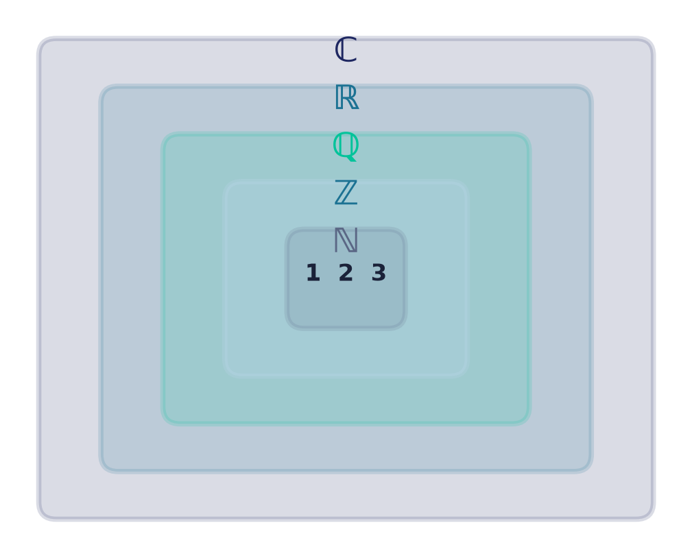
These sets nest inside one another:
Every natural number is an integer, every integer is rational (e.g. ), every rational is real, and every real is complex (with imaginary part ). Each inclusion is proper — there are integers that are not natural (), rationals that are not integers (), reals that are not rational (), and complexes that are not real ().
Example 1.6 (classification). Classify .
- (and hence also in ).
- but .
- but .
- (irrational) but .
- (in fact ) but .
The blackboard-bold letters denote the smallest customary system; each number also lives in every larger system in the chain.
Intervals of
Subsets of the real line are named by interval notation. For : the closed interval includes both endpoints; the open interval excludes both; the half-open and include exactly one; and the rays , (and their variants) are unbounded. A square bracket means the endpoint is in the set, a round bracket that it is not; always takes a round bracket. This notation is used throughout the course — e.g. for a probability, for a function’s domain.
3.1 A worked proof: is irrational
That the chain is proper is not obvious — one must produce a real number and prove it is not a ratio of integers. The classic example is . The proof, known to the Pythagoreans around 500 BCE, is a model of the technique proof by contradiction.
Theorem 1.7. is irrational; that is, there are no integers with and .
Proof. Suppose, for contradiction, that is rational. Then we may write with , , and the fraction in lowest terms, i.e. (any fraction can be reduced to lowest terms by cancelling common factors). Squaring gives , hence
Equation says is even. Now even forces even: for if were odd, say , then would be odd. So is even; write . Substituting into :
By the same reasoning is even, so is even. But now and , contradicting . The assumption that is rational is therefore untenable, and is irrational. ∎
Remark. The same argument shows is irrational whenever is a natural number that is not a perfect square. The proofs that and are irrational are far harder and belong to analysis; we cite them but do not prove them here.
Historical note. The discovery that the diagonal of a unit square (length ) is incommensurable with its side shattered the Pythagorean belief that all magnitudes are ratios of whole numbers. It is one of the earliest known proofs by contradiction and one of the first genuine theorems about the structure of the number line.
1.4 Subsets and inclusion
4.1 The definition
Definition (subset). is a subset of , written , when every element of is also an element of :
If in addition — i.e. has at least one element not in — we call a proper subset of and write (some texts write to stress properness).
Intuitively says “ fits inside .” The definition is a universally quantified conditional, and that logical shape dictates how we prove inclusions: to prove , take an arbitrary and derive . This “take an arbitrary element” move is the single most common opening line in set-theoretic proofs.
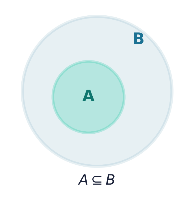
Example 1.8. Let and . Every element of ( and ) lies in , so ; and since but , the inclusion is proper: . By contrast, because — a single “witness” element outside suffices to refute an inclusion.
Common pitfall ( vs. ). These are different relations. With : (true), (true), but is a type error ( is not a set) and is false (’s elements are and , not the set ). The traps get sharper with nested sets: for we have and , but and .
4.2 The empty set is a subset of everything (vacuous truth)
Our first structural theorem is one students often find surprising, because it seems to say “nothing is inside everything.” The resolution is the logical principle of vacuous truth: a conditional whose hypothesis is false is counted as true, regardless of . (Compare an unfulfillable promise: “if you finish a marathon in hour, I’ll pay you 1000 dollars” is never broken if no such marathon is ever run.) Vacuous truth is developed fully in the propositional-logic material; here we use it.
Proposition 1.9. For every set , .
Proof. By definition we must show . Let be arbitrary. The hypothesis “” is false, because the empty set has no elements. A conditional with a false hypothesis is true (vacuous truth). Hence holds for this — and therefore every — . Thus . ∎
Alternative proof (by contradiction). Suppose . By the definition of , this failure means there exists an element with and . But is impossible. This contradiction shows . ∎
The second proof is worth studying: it shows how to negate a subset claim. The negation of “” is “.” To disprove you exhibit one such witness ; to prove it you rule all witnesses out.
4.3 Reflexivity and transitivity of
Proposition 1.10 (reflexivity). For every set , .
Proof. For every , the conditional is true (a statement implies itself). Hence . ∎
Proposition 1.11 (transitivity). If and , then .
Proof. Let be an arbitrary element of . Since , from we get . Since , from we get . Thus every element of is an element of , i.e. . ∎
Remark (a preview of order theory). Propositions 1.10, 1.11 and Theorem 1.13 (antisymmetry) together say that is a partial order on any collection of sets: reflexive, antisymmetric, and transitive. Partial orders are studied systematically in the lecture on relations (Lecture 3); the power set ordered by is the prototypical example and reappears in the lecture on Boolean algebras and lattices.
Example 1.12. , so by transitivity — as is directly visible. Transitivity earns its keep in proofs where the intermediate set is not something you would want to compute element-by-element.
1.5 Set equality and the double-inclusion method
5.1 Extensionality
When are two sets equal? The guiding principle, called the axiom of extensionality, is that a set is nothing more than its members:
Definition / Axiom (extensionality). Two sets are equal, , exactly when they have the same elements:
Extensionality is why order and repetition inside braces do not matter (§1.1): and have the same members, hence are equal. It also means sets described in totally different ways can turn out equal — and proving such equalities is a core skill.
5.2 The double-inclusion criterion
The biconditional “” splits into two conditionals, and those two conditionals are precisely two subset statements. This yields the workhorse theorem of the whole chapter.
Theorem 1.13 (equality via double inclusion; antisymmetry of ). For all sets ,
Proof. () Suppose . By extensionality, for every we have . In particular (so ) and (so ).
() Suppose and . Let be arbitrary. From we have ; from we have . Combining the two conditionals, . As was arbitrary, and have the same elements, so by extensionality . ∎
The double-inclusion proof template. To prove two sets and are equal:
- () Assume ; through valid steps deduce . Conclude .
- () Assume ; through valid steps deduce . Conclude .
- By Theorem 1.13, . ∎
This template appears constantly in Lecture 2, where every set identity (De Morgan’s laws, distributivity, absorption, …) is proved this way.
5.3 Worked examples of set equality
Example 1.14 (order and repetition). . All three descriptions list exactly the members ; by extensionality they denote one set.
Example 1.15 (double inclusion, roster vs. set-builder). Let and . We claim .
Proof. () Let . Then and , so , i.e. ; hence or . In either case . Thus . () and , so ; likewise , so . Hence . By double inclusion, . ∎
Example 1.16 (two set-builder descriptions). Let
We claim (both are “the even integers”).
Proof. () Let , so for some . Then is even, so . () Let , so is even. If were odd, then would be odd (§1.3.1); since is even, must be even, i.e. for some , so . Hence , and . ∎
Example 1.17 (unequal sets — refute one inclusion). , because belongs to the first set but not the second, so the inclusion fails. To show inequality it is enough to break one of the two inclusions.
Example 1.18 (element vs. singleton, revisited). : the left side is a number, the right side is a set. Likewise : the left side’s element is , the right side’s element is , and .
Common pitfall (proving equality with only one inclusion). A frequent error is to prove and stop, concluding . One inclusion gives only “ is part of ,” which is consistent with . Both directions are needed. Conversely, when the two directions have identical-looking steps, say so explicitly (“by the symmetric argument”) rather than omitting a direction.
1.6 Ways to describe a set
There are three standard ways to specify which elements a set contains.
6.1 Roster (list) notation
List the elements explicitly between braces, e.g. . For a clear, unambiguous pattern an ellipsis is permitted: or . Roster notation is only practical when the set is small or its pattern is obvious.
6.2 Set-builder (predicate) notation
Describe the elements by a property (predicate) they must satisfy:
Almost always a domain is supplied to keep the definition safe and definite (§1.12 explains why this matters):
This separation form carves out of exactly the elements satisfying .
Notation. The bar is read “such that.” Some texts — and a few later sections here — write a colon instead, ; the two are interchangeable.
A second, closely related form specifies elements by an expression ranging over a domain — the image or replacement form:
Here the bar separates a rule for producing elements (left) from the range of the input (right).
Example 1.19. The roster equals the set-builder description .
Example 1.20 (roster impossible). is the open interval . Roster notation cannot express it (uncountably many elements — §1.9), so set-builder notation is essential, not merely convenient.
Example 1.21 (empty via unsatisfiable predicate). , since no real number squares to a negative value. A set-builder description names precisely when its predicate is unsatisfiable over the domain.
Example 1.22 (congruences). , the integers leaving remainder on division by . Such sets (residue classes) reappear in the number-theory and modular-arithmetic material.
Example 1.23 (a set of pairs). is the unit circle in the plane. Set-builder notation ranges naturally over tuples (§1.11), which is how curves, relations, and graphs get defined.
Example 1.24 (the rationals). . Note this uses the image form; many different pairs name the same rational (), which is fine — extensionality collapses the duplicates.
Common pitfall (unrestricted comprehension). Writing with no domain — quantifying over “all objects whatsoever” — is dangerous. Taking to be “” produces Russell’s paradoxical set (§1.12). Modern set theory only permits the separation form , carving from a set already known to exist. In this course, always give the domain.
6.3 Recursive (inductive) definition
Give base elements and rules that generate new elements from old ones. This third style is important enough — and central enough to computer science — to get its own section.
1.7 Recursive (inductive) definitions
7.1 Motivation and the three parts
How do you define an infinite set precisely, using only finitely many words, without a closed formula? You bootstrap: declare a few elements outright, then give rules that manufacture new elements from ones you already have. This is exactly how programmers define linked lists (“a list is empty, or a head followed by a list”), how compilers define the syntax of expressions, and how logicians define formulas.
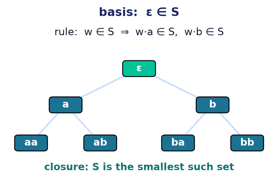
Definition (recursive/inductive definition). A recursive definition of a set has three parts:
- a base case (basis) — one or more elements declared to be in outright;
- a recursive rule (induction step) — how to build new elements of from elements already known to be in ;
- a closure clause — contains nothing except what the basis and rules force (usually left implicit).
The closure clause matters: without it, “the set containing and closed under ” could be or all of or all of . Closure makes the smallest set satisfying the basis and rule.
7.2 Examples
Example 1.25 (positive even numbers). Define by basis ; rule if then . Applying the rule repeatedly gives , so .
Example 1.26 (powers of two). Basis ; rule if then . This generates .
Example 1.27 (strings over an alphabet). Fix a finite alphabet (e.g. ). The set of all finite strings is defined by basis the empty string ; rule if and then the concatenation . This is the founding definition of formal-language theory (used heavily in the lectures on regular languages and automata): a language is then simply a subset of .
Example 1.28 (balanced parentheses / the Dyck language). Over
, define by: basis ; rules if
then , and if then . Then
is exactly the set of correctly-nested parenthesis strings: , (),
(()), ()(), (()()), … Recursively-defined languages like this are what
parsers recognize.
Example 1.29 (arithmetic expressions). Over operands and operators : basis each of is an expression; rule if and are expressions then so are and . This generates all fully-parenthesized expressions such as — the abstract syntax that every compiler builds.
Example 1.30 (binary trees). Basis the empty tree is a binary tree; rule if and are binary trees then the ordered triple (left subtree, root, right subtree) is a binary tree. Data structures are recursively-defined sets; this is why they pair so naturally with recursion and induction in code.
Remark (structural induction). Every recursively-defined set comes with a matching proof method: to show every element of has a property , prove holds for the basis elements and is preserved by each rule. This is structural induction, the generalization of ordinary induction on , developed in the lecture on mathematical induction. For instance, one proves “every string in the Dyck language has equally many
(and)” by structural induction on the definition in Example 1.28.
Remark (the natural numbers are themselves recursive). Even can be built recursively. In the von Neumann construction one sets and , so
Each number is the set of all smaller numbers, so . This shows sets are expressive enough to encode the counting numbers themselves — the whole of mathematics can, in principle, be founded on the single relation .
1.8 Cardinality — the “power” of a set
8.1 Counting elements
Definition (cardinality). The cardinality of a set , denoted , is the number of elements it contains. A set is finite if for some , and infinite otherwise.
(In older texts and the course deck, cardinality is called the power of a set — Cantor’s original German term was Mächtigkeit. The unrelated “power set” of §1.10 borrows the same word.)
- .
- .
- — duplicates are not counted twice (extensionality).
- — two distinct elements.
Example 1.31. For we have . For we have as well. So even though : cardinality measures how many, not which.
8.2 Equinumerosity: comparing sizes with bijections
Example 1.31 hints at the deep idea that drives the rest of this chapter: two sets have the “same size” when their elements can be matched up one-to-one, with none left over on either side. This matching idea — not counting — is what generalizes to infinite sets.
Definition (equinumerous). Sets and are equinumerous, written , if there is a bijection (a function that is both injective — no two inputs share an output — and surjective — every output is hit). We write if there is an injection .
For finite sets this agrees with ordinary counting. Its power is that it needs no notion of “number” at all, so it applies to infinite sets, where it produces genuinely surprising results (§1.9). Functions, injectivity, surjectivity, and bijectivity are defined here as we need them, as counting tools; functions in their own right appear as a special kind of relation in Lecture 3 (§3.12).
Remark. Exhibiting a bijection is the gold-standard way to prove two sets have equal size — you will see it used to prove in §1.10 and in §1.11, and it underlies the combinatorial “bijective proofs” in the combinatorics of Lecture 13.
1.9 Countable and uncountable sets
9.1 Are all infinities the same size?
Here is one of the most beautiful discoveries in mathematics, due to Georg Cantor (1870s–1880s): there are different sizes of infinity. The infinite set can be matched one-to-one with and even with , but cannot be matched with — the reals are strictly more numerous. We sketch why. These facts are not needed arithmetically in the rest of the course, but the distinction between countable and uncountable is genuinely used: e.g. the set of all programs is countable while the set of all functions is uncountable, which is the seed of the existence of uncomputable functions (a theme of the computability material).
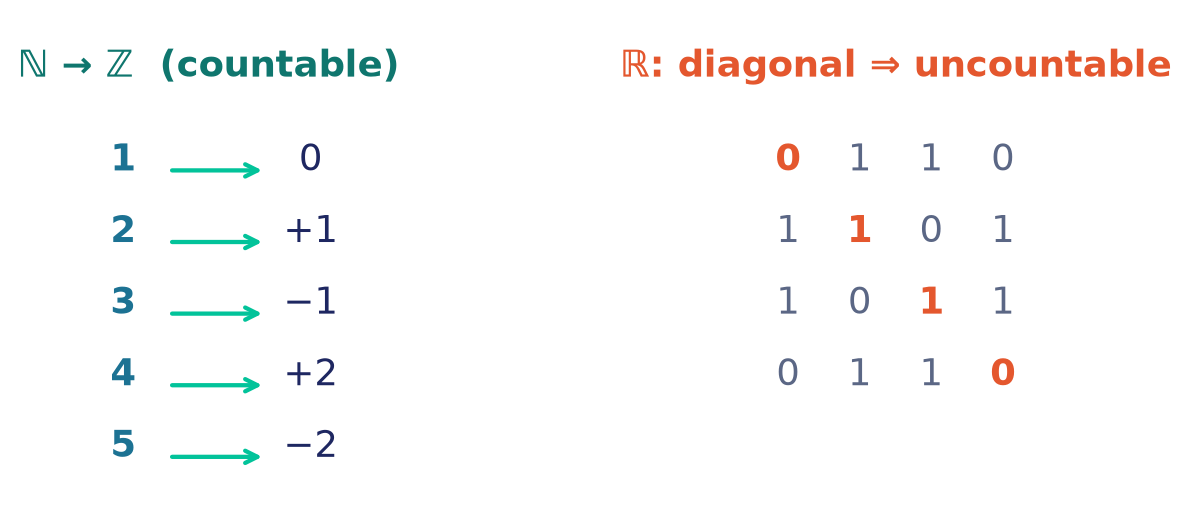
Definition (countable / uncountable). A set is countably infinite if , i.e. there is a bijection — equivalently, ’s elements can be arranged in an infinite list with each element appearing exactly once. A set is countable if it is finite or countably infinite, and uncountable otherwise. The cardinality of is written (“aleph-null”).
9.2 and are countable
Theorem 1.32. is countably infinite.
Proof. We exhibit a bijection by listing the integers so that each appears exactly once:
Explicitly, if is even, and if is odd (recall ). Then Every integer appears exactly once — the non-positive integers at odd inputs, the positive integers at even inputs — so is a bijection. Hence . ∎
The lesson is counterintuitive: “looks twice as big” as , yet the two are equinumerous. With infinite sets, a proper subset can have the same cardinality as the whole (indeed this is a characterization of infinity).
Theorem 1.33 (Cantor). is countably infinite.
Proof sketch. Arrange the positive rationals () in an infinite grid, row and column :
Traverse the grid along successive anti-diagonals (), skipping any fraction not in lowest terms (so each rational is counted once). This lists every positive rational: is countable. Now interleave with and the negatives — — to list all of . Hence is countably infinite. ∎
The same anti-diagonal “dovetailing” shows that a countable union of countable sets is countable, and that is countable — facts reused throughout computer science (e.g. enumerating all pairs, all strings, all programs).
9.3 is uncountable: Cantor’s diagonal argument
Now the punchline: no list can exhaust the reals.
Theorem 1.34 (Cantor, 1891). The interval is uncountable. Consequently is uncountable.
Proof (diagonalization). Suppose, for contradiction, that is countable. Then its elements can be listed as a sequence containing every number in . Write each in decimal:
where is the -th decimal digit of . Now construct a new number by altering the diagonal digits (shown in bold):
By construction , and for every . Therefore differs from in the -th decimal place, for every , so for all . But the list was supposed to contain every element of , and — contradiction. Hence cannot be listed: it is uncountable. Since , the larger set is uncountable as well. ∎
Remark (why the digits and ). A real number can have two decimal expansions only when one ends in all $9$s and the other in all $0$s (e.g. ). We chose precisely so that uses no $0$s or $9$s; hence has a unique decimal expansion, and the guarantee “ differs from at digit ” cannot be voided by an alternate expansion of . This care is what makes the argument airtight rather than merely suggestive.
Remark (the continuum). Cantor’s argument shows : the reals form a strictly larger infinity, the continuum. So the “gap” between and that Theorem 1.7 opened for the single number is in fact enormous — the irrationals are uncountable, while the rationals we can list are, in this precise sense, negligibly few.
9.4 Cantor’s theorem: the power set is always bigger
Diagonalization is not a trick special to decimals; it is a general phenomenon.
Theorem 1.35 (Cantor’s theorem). For every set , there is no surjection . Consequently — a set always has strictly fewer elements than its power set, even when is infinite.
Proof. Let be any function; we show misses some subset. Define the “diagonal” set
Suppose were in the image of , say for some . Ask whether . By the definition of ,
since . Thus “” holds iff it fails — a contradiction. So no such exists, is not in the image of , and is not surjective. As no surjection exists (while is an injection ), we conclude . ∎
Taking yields , so is uncountable (in fact ). Iterating, : there is no largest infinity. Notice, too, how the diagonal set in this proof is the very same self-referential construction that produces Russell’s paradox in §1.12 — the two are the same idea wearing different clothes.
Historical note. Cantor’s creation of set theory and his hierarchy of infinities were revolutionary and, at first, fiercely resisted. Today his diagonal method is a cornerstone not only of set theory but of computability (the undecidability of the halting problem is a diagonal argument) and of logic (Gödel’s incompleteness theorems).
1.10 The power set
10.1 Definition and examples
Since subsets of a set are themselves objects, we may collect all of them into a new set.
Definition (power set). The power set of , written (also or ), is the set of all subsets of :
Its elements are themselves sets. Both and always belong to (by Proposition 1.9 and 4.2).
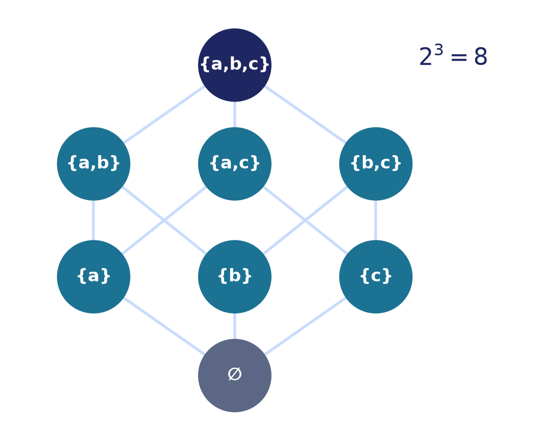
Example 1.36. — one element (not zero!), so . And , with . And , with .
Example 1.37 (from the deck). For , the power set has members:
Grouped by size: one subset of size , four of size , six of size , four of size , and one of size — a total of .
Common pitfall. , not : the empty set has exactly one subset, namely itself. Similarly for every , so is never empty even when is.
10.2 The size of the power set
The grouping in Example 1.37 (with row sums — the binomial coefficients ) points to the central theorem. We give two independent proofs, because each teaches a reusable technique.
Theorem 1.38. If is finite with , then .
Proof 1 — by a bijection with bit-strings
Proof. List the elements as . Let be the set of length- bit-strings (ordered -tuples of $0$s and $1$s). Define by sending each subset to its characteristic vector
We show is a bijection.
- Injective. Suppose . Then for each , . So and contain exactly the same , i.e. .
- Surjective. Given any bit-string , form . Then . So every bit-string is hit.
Hence is a bijection, and . Finally : a length- bit-string is built by choosing each of the coordinates independently from options, so by the product rule (Lecture 13’s combinatorics) there are of them. Therefore . ∎
This bijection is not merely a counting device — it is how sets are stored in computers (§1.11.4 / §1.13): a subset of an -element universe is a single -bit word.
Proof 2 — by induction on
Proof. We induct on .
Base case (). The only set with elements is , and , so . ✓
Inductive step. Assume (induction hypothesis) that every set with elements has exactly subsets. Let be any set with . Fix an element and put , so . Split the subsets of into two classes according to whether they contain :
- Subsets not containing . These are precisely the subsets of . By the induction hypothesis there are of them.
- Subsets containing . Each has the form for a unique , and conversely each yields one such subset. This pairing is a bijection with the subsets of , so again there are .
The two classes are disjoint (a set either contains or not) and together exhaust . By the sum rule,
This completes the inductive step. By the principle of mathematical induction, for all . ∎
Remark (why prove it twice). The bijective proof gives insight — subsets “are” bit-strings — and generalizes to a formula-free count. The inductive proof models the standard “fix one element, split into two cases” strategy that recurs across combinatorics. Meeting both now prepares you for the combinatorics of Lecture 13.
Corollary 1.39 (a binomial identity). For every ,
Proof. Classify the subsets of an -set by their size . The number of -element subsets is (this is the definition of the binomial coefficient, established in the combinatorics of Lecture 13). Summing over all possible sizes counts every subset exactly once, which by Theorem 1.38 totals . ∎ For this reads , matching Example 1.37 exactly.
Remark (the notation ). The alternative symbol for the power set is deliberate: writing , the set of all functions is (via characteristic functions) the set of subsets of , and its size matches. This viewpoint also gives meaning to for infinite : , the continuum of §1.9.
10.3 The power set and the set operations
The power set interacts cleanly with the operations of Lecture 2. For all sets :
- — a set is a subset of both and exactly when it is a subset of ;
- , and the inclusion is usually strict: but lies in neither nor ;
- — monotonicity, since then forces , i.e. .
Each is a one-line element-chase: rewrite “” as “” and unfold the definitions of .
1.11 Ordered pairs, tuples, and the Cartesian product
11.1 When order matters
Sets deliberately forget order, but a great deal of mathematics and computing needs
to remember it: the point in the plane is not ; the database row
("Ada", 1815) pairs a name with a year in a fixed layout; a function’s input
output pairing is directional. For this we use ordered pairs.
Definition (ordered pair). An ordered pair records a first component and a second component . Its defining property is that order is significant:
In particular , whereas the sets and are equal. Repetition is allowed in a pair: is perfectly valid, though as a set.
Remark (pairs are secretly sets — Kuratowski). Ordered pairs need not be a new primitive; they can be encoded as sets. Kuratowski’s definition is
One can prove from this that , recovering exactly the defining property. This is a recurring theme: with enough ingenuity, every discrete structure (pairs, numbers, functions, relations) can be built out of plain sets and the single relation . We will use pairs as if primitive and never unfold the encoding.
Definition (-tuple). For , an -tuple is an ordered list of components. Two -tuples are equal iff they agree in every coordinate:
Ordered pairs are the case ; a -tuple locates a point in space.
11.2 The Cartesian product
Definition (Cartesian product). The Cartesian product of sets and is the set of all ordered pairs with first component from and second from :
More generally, , and abbreviates ( factors).
The name honors René Descartes, whose coordinate geometry identifies the plane with and space with .
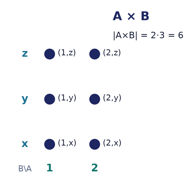
Example 1.40. With and , a typical element of is , and even though both pairs live in . Here (Proposition 1.42).
Example 1.41 (product need not be square). With and ,
so . Note in general (their elements are pairs in opposite orders), so the Cartesian product is not commutative — one of several algebraic facts developed in Lecture 2.
11.3 Counting the product
Proposition 1.42. For finite sets, .
Proof. Let with and . Partition according to the first coordinate:
These blocks are pairwise disjoint (pairs with different first coordinates are different), and each block is in bijection with via , so each has exactly elements. By the sum rule, . ∎
By induction this extends to ; in particular . For instance , recovering the bit-string count used in Theorem 1.38.
Remark (cross-reference). The Cartesian product is the stage on which relations and functions are defined: in Lecture 3, a relation from to is any subset , and a function is a relation in which each appears as a first coordinate exactly once. Thus everything in this section is prerequisite machinery for the two lectures that follow.
11.4 A first glimpse of applications
The three constructions of this chapter map cleanly onto everyday computing objects:
- a subset of a fixed finite universe ⟷ a bit-set / bitmask (§1.13.1);
- a tuple ⟷ a record / struct / row (§1.13.2);
- a Cartesian product ⟷ the type of all such rows (§1.13.2–13.3).
§1.13 develops these.
1.12 Russell’s paradox and a note on axioms
12.1 The paradox
The naive rule we have used informally — “any property determines the set of all objects with that property” — is called unrestricted comprehension. In 1901 Bertrand Russell noticed it is self-contradictory.
Some sets are members of themselves and some are not — under naive comprehension, at least; e.g. “the set of all sets” would contain itself. Consider the property “ is not a member of itself,” and form the set it supposedly determines:
Now ask the fatal question: is ?
- If , then satisfies the defining property, i.e. .
- If , then satisfies the defining property, so .
Either way we reach , an outright contradiction. So no such set can exist, and unrestricted comprehension is untenable. (The kinship with Cantor’s diagonal set in Theorem 1.35 is exact: both hinge on an object asked whether it belongs to a set defined by not belonging.)
A homelier version — the barber. In a certain village the barber shaves exactly those men who do not shave themselves. Does the barber shave himself? If he does, he shouldn’t; if he doesn’t, he must. The “barber” cannot exist — just as the set cannot.
12.2 The resolution
The fix is to forbid conjuring sets out of properties alone. Modern set theory (the Zermelo–Fraenkel axioms, ZF/ZFC) replaces unrestricted comprehension with the axiom schema of separation: from an already existing set you may carve
but you may not form over the whole universe. Because the paradoxical needs to range over all objects, it is never constructed, and the contradiction disappears. There is also, provably, no set of all sets in ZFC — which is why §1.2 insisted the universal set is always a concrete set fixed by context, never “everything.”
This is exactly why, throughout this course, we write set-builder expressions with a domain: , . The habit is not pedantry — it is the discipline that keeps set theory consistent.
Historical note. Russell communicated the paradox to Gottlob Frege in 1902, just as the second volume of Frege’s Grundgesetze der Arithmetik — which sought to found all of arithmetic on unrestricted comprehension — was in press. Frege’s stricken reply conceded the foundation had collapsed. The repair by Ernst Zermelo (1908) and Abraham Fraenkel (1920s) produced the ZFC axioms on which essentially all of contemporary mathematics is now built.
1.13 Applications in computer science
Sets are not just notation; the constructions above are implemented directly in hardware, databases, and programming languages.
13.1 Bit-sets (bitmasks)
Fix a universe of items indexed . By the characteristic-vector bijection of Theorem 1.38, every subset corresponds to a length- bit-string, which fits in a machine integer (an -bit word). Set operations become single hardware instructions on that word:
| Set concept | Bit operation | Cost |
|---|---|---|
test bit : (w >> i) & 1 |
||
bitwise OR a | b |
per word | |
bitwise AND a & b |
per word | |
| (complement in ) | bitwise NOT ~a |
per word |
a & ~b |
per word | |
| $ | A | $ (cardinality) |
This is why a -element universe is a natural unit: one subset per uint64.
Bit-sets power register allocators, graph reachability, chess engines
(“bitboards”), and the fast set operations behind search engines. Every identity we
prove about in Lecture 2 is simultaneously a
theorem about these bit operations (the shared abstraction is Boolean algebra).
13.2 Relational databases
A database table with columns of types has rows that are -tuples in the Cartesian product . The table itself is a finite subset of that product — i.e. exactly a relation (Lecture 3):
Because rows form a set, duplicate rows collapse (extensionality) and row order is
irrelevant — matching SQL’s SELECT DISTINCT and the fact that query results are
unordered unless you add ORDER BY. The operations of relational algebra — union,
intersection, difference, projection, selection, join — are set operations on these
subsets of Cartesian products, so this lecture and Lecture 2 are the direct
mathematical foundation of SQL.
13.3 Type systems and algebraic data types
In a typed programming language a type can be understood as the set of its values, and the type constructors mirror set constructions — the reason they are called algebraic data types:
| Type construct | Set analogue | Cardinality |
|---|---|---|
product / struct / record / tuple (A, B) |
||
sum / variant / enum / tagged union A + B |
disjoint union | |
function type A -> B |
set of functions | |
unit type () |
singleton | |
empty / Void type |
For example, the type Bool = {true, false} has cardinality ; a pair
(Bool, Bool) has values; and Bool -> Bool has
functions — precisely . Counting a type’s inhabitants (its cardinality)
tells you, for instance, how many cases a switch must handle to be exhaustive, and
the isomorphisms of this algebra (e.g. , )
justify refactorings compilers perform automatically.
13.4 Formal languages (preview)
By Example 1.27 the set of strings over an alphabet is recursively defined, and a language is any subset . Since is countably infinite, it has uncountably many subsets (Theorem 1.35), so there are uncountably many languages — but only countably many finite descriptions (programs/grammars). By a counting argument, most languages have no finite description: an early hint, grounded entirely in this chapter, that uncomputable and undecidable problems must exist. This thread is picked up in the lectures on regular languages, automata, and computability.
Chapter summary
Set theory supplies the vocabulary for the entire course. A set is an unordered collection of distinct elements, fully determined by its members (extensionality), so order and repetition inside braces are invisible. Membership is the single primitive relation. Two sets among all others are singled out: the empty set , which we proved is unique and is a subset of every set (by vacuous truth), and a context-dependent universe — never “everything,” lest Russell’s paradox strike.
We compare sets with inclusion , a partial order (reflexive, transitive, antisymmetric), and we prove two sets equal by the double-inclusion method — showing each contains the other — which is the template for every set identity to come. Sets are described three ways: by roster, by set-builder predicate (always over a stated domain, to stay safe), and by recursive definitions with a basis, a rule, and a closure clause — the last being how computer science defines strings, expressions, and data structures, and the natural partner of proof by (structural) induction.
We measure sets by cardinality , comparing sizes via bijections. This idea scales to the infinite, where Cantor’s results overturn intuition: and are countable, but is uncountable by the diagonal argument, and for every set. The power set of all subsets satisfies when , which we proved twice — bijectively (subsets bit-strings) and by induction. Finally, ordered pairs, tuples, and the Cartesian product (with ) restore the notion of order and set the stage for relations and functions. The same three constructions reappear as bit-sets, database tables, and program types.
Key facts.
- Extensionality: ; order and repetition are irrelevant.
- is unique, , and for every (vacuous truth); but and .
- Numeric hierarchy: , each inclusion proper; .
- ; is reflexive, transitive, antisymmetric.
- Equality by double inclusion: .
- Descriptions: roster, set-builder , recursive (basis + rule + closure).
- ; .
- Countable: . Uncountable: , . Always (Cantor).
- ; ; product is not commutative.
- Never form without a domain (Russell’s paradox).
Exercises
Warm-up
1. State the two principles (order, repetition) that make , , and all denote the same set. What single axiom underlies both?
2. Explain the difference between , , and . Give the cardinality of each.
3. Place each of into the smallest customary numeric set () that contains it.
4. For , decide each of: ; ; ; ; ; ; .
5. Is a proper subset of ? Is it a subset? Justify both answers.
6. Compute for and list all of its elements grouped by size.
7. Why is while ? How many elements does have when and ?
Standard
8. Prove by double inclusion that .
9. Rewrite in set-builder notation, and give a recursive definition (basis + rule) of the set of all positive multiples of .
10. Let and . Prove .
11. Prove that for all sets, and imply (transitivity), taking arbitrary elements explicitly.
12. List all elements of , and separately of . Are the two products equal? What does this show about commutativity of ?
13. Using the recursive definition of the Dyck language (Example 1.28), list all balanced-parenthesis strings of length , and state how many there are of length exactly .
14. A byte is a bit-string of length . Using the characteristic-vector idea, explain why there are exactly subsets of an -element universe, and describe which byte represents the subset of .
Challenge
15. Prove that is irrational. Where exactly does the proof use that is prime (equivalently, not a perfect square)?
16. Prove carefully that for every set by contradiction, writing out the negation of “” explicitly before deriving the contradiction.
17. Give the two proofs that (bijection with bit-strings; and induction on ) in your own words. In the inductive step, identify precisely where the induction hypothesis is used.
18. Prove that the set is countable by describing an explicit listing (e.g. by anti-diagonals). Then explain in one or two sentences why the same style of argument fails to list the reals in .
19. (Cantor’s theorem, hands-on.) Let and let be . Compute the diagonal set and verify explicitly that for every .
20. Explain why the set cannot exist. Then explain in one sentence how the ZFC separation axiom (, with a set) blocks the paradox.
Selected answers & hints
2. (no elements); (one element, namely ); (one element, the number ). All three are different objects: an empty box, a box holding an empty box, and a box holding the number zero.
4. True: , , , . False: (the object is not an element of ; it only appears inside elements), (this would need , which is false), (needs ). Moral: distinguish from , and do not “see through” braces.
5. is true (reflexivity, Prop. 4.2: every element of the left is in the right). It is not a proper subset, because properness requires the two sets to differ, and here they are equal.
6. : ; ; ; — grouped .
8. () If and then , so or ; either way . () and with , so both belong to the left set. Hence equality by double inclusion.
9. . Recursive definition of all positive multiples of : basis ; rule if then ; (closure).
12. ; . Both have elements, but the products are not equal (e.g. is in the first, not the second), so is not commutative.
13. Length : . Length : (). Length : (()), ()() —
two of them. (Odd lengths are impossible.) The count of balanced strings of length
is the Catalan number ; for length (), .
14. Each of the elements is independently in or out, giving characteristic vectors, hence subsets. With bit meaning “,” the subset is the byte (bit leftmost) — equivalently value .
15. Mimic Theorem 1.7: assume in lowest terms, get , so . Primality of gives (a prime dividing a product divides a factor — Euclid’s lemma; this is the step that needs prime). Write , deduce , contradicting lowest terms. (For a non-square like , , the argument works; for a perfect square like it correctly fails, since is rational.)
16. Negation of : “.” Such an satisfies , impossible. The existence assumption is therefore false, so .
18. List by anti-diagonals: , i.e. group pairs by the constant sum ; each group is finite, so concatenating them enumerates all pairs — a bijection with . It fails for because a real is an infinite sequence of digits, not a finite pair of indices; the diagonal argument (Thm 9.3) shows any purported list is incomplete.
19. , so ; , so ; , so . Thus . Checking: , , — none equals , so is outside the image of , confirming is not surjective.
20. If existed, then (substitute into the defining property), a contradiction; so cannot exist. Separation only lets you form for an already-existing set ; the result is a subset of and one shows it simply is not an element of , producing no contradiction — the self-swallowing “set of all sets” is never available.
Further reading
- Kenneth H. Rosen, Discrete Mathematics and Its Applications — Chapter 2 (Basic Structures: Sets, Functions, Sequences, Sums, and Matrices) covers sets, the power set, and Cartesian products, and §1.2.5 treats cardinality and Cantor’s diagonal argument.
- Susanna S. Epp, Discrete Mathematics with Applications — Chapter 6 (Set Theory) develops the element method for proving subset and equality relations in careful detail, closely matching the double-inclusion technique of §1.5.
- For the axiomatic and historical background (extensionality, separation, Russell’s paradox, ZFC), Paul Halmos’s Naive Set Theory is a classic short treatment.
These texts use in places; recall (§1.3) that our course convention is .