Lecture 3. Relations
Learning objectives
After studying this chapter you should be able to:
- state precisely what a binary relation and an -ary relation are, and move fluently between the three standard representations (set of pairs, Boolean matrix, digraph);
- recognise and prove the structural properties of a relation — reflexive, irreflexive, symmetric, antisymmetric, asymmetric, transitive — including their algebraic characterisations (, , , );
- compute inverses and compositions, and justify why composition is realised by the Boolean matrix product and why it is associative;
- construct the reflexive, symmetric and transitive closures of a relation, prove the formula , and explain why the union is finite on a finite set;
- prove the Fundamental Theorem of Equivalence Relations (equivalence relations partitions) in both directions and apply it to congruence classes in modular arithmetic;
- analyse partial orders: comparability, Hasse diagrams, minimal/maximal and least/greatest elements, bounds, and a first look at lattices;
- connect the theory to computer science, especially the relational database model and relational algebra.
This chapter builds directly on Lecture 1 (subsets, power sets) and Lecture 2 (set operations, ordered tuples, and the Cartesian product). It is used later whenever we group outcomes into cases — for example in Lecture 13, where an equivalence relation on a sample space partitions it into the disjoint events that make counting and probability tractable.
3.1 Overview and motivation
Sets on their own describe collections of objects, but almost every interesting mathematical or computational statement is about how objects are linked: “ is less than ”, “student received mark in subject ”, “city has a direct flight to city ”, “web page links to page ”, “process must run before process ”. A relation is the mathematical object that captures exactly this idea of a link between elements — nothing more and nothing less.
The whole subject rests on one deceptively small idea from Lecture 2: an ordered pair remembers not only which two objects are involved but also which comes first. (Recall Kuratowski’s set-theoretic encoding , which makes hold iff and .) A relation is then simply a set of such pairs selected out of a Cartesian product. Everything else in this chapter — matrices, digraphs, equivalence classes, orders, database tables — is a consequence of taking that one definition seriously.
Three themes recur throughout:
- One object, several faces. A relation is simultaneously a set of tuples, a Boolean matrix, and a directed graph. Each face makes some questions trivial: the matrix face turns “is there a two-step path?” into arithmetic; the graph face makes reachability visible; the set face makes union/intersection obvious.
- Structure via properties. A handful of properties (reflexive, symmetric, transitive, …) carve out the two most important species of relation: equivalence relations, which formalise “the same for our purposes”, and partial orders, which formalise “ranking, possibly with ties left incomparable”.
- From theory to systems. The generalisation to -ary relations is not an afterthought: it is literally the data model of every relational database, and the set operations of Lecture 2 reappear as the core of relational algebra and hence of SQL.
3.2 Tuples and the Cartesian product (recap from Lecture 2)
A tuple is an ordered list of elements. Given sets , an ordered triple is written with , , ; order matters and repetition is allowed, distinguishing tuples from sets. The Cartesian product collects all such tuples:
For finite sets the product rule gives .
Example. With , , we get triples:
The Cartesian product is the “universe” of all conceivable tuples; a relation picks out the tuples we actually care about.
Remark (why order and repetition matter). The pair is not the pair , and is a perfectly good pair even though the set collapses. This is precisely why relations can express asymmetric links such as “ is the parent of ” that a symmetric set-of-two could never record.
3.3 Binary relations as subsets of a Cartesian product
Definition 3.1 (binary relation). A binary relation from a set to a set is any subset . When we say is a relation on (so ). Its elements are ordered pairs .
Two notations mean exactly the same thing:
read “ is related to ”. They are interchangeable because is its set of pairs — the infix statement is only shorthand for membership in that set. The infix form mirrors the familiar or and is usually more readable; we shall use whichever is clearer.
There are two standard ways to specify a relation:
- By listing the ordered pairs explicitly (an extensional definition), and
- By a predicate, i.e. a defining property (an intensional definition): .
Example 3.2 (both ways, one relation). Let and let be “strictly less than”. Extensionally,
intensionally,
Both describe the same six pairs. The intensional form scales to infinite sets (the relation on ) where listing is impossible.
More examples of the infix form .
- “less than or equal to”: , , .
- “is divisible by”: , , .
- “uses the same digits as”: , , (both sides use only the digits ).
Common pitfall (a relation is not a rule). A relation need not be describable by any tidy formula. On the set is a perfectly legitimate relation even though no arithmetic condition singles out those three pairs. Conversely, do not confuse the predicate with the relation: two different predicates ( and “ is a positive integer”) can define the same relation.
3.4 Domain and range
For :
Definition 3.3. The domain of is — the first components that actually occur. The range (or image) of is — the second components that actually occur.
Example 3.4. For the “strictly less than” relation of Example 3.2, (the value is less than nothing in ) and (nothing is less than ). Both are subsets of ; neither need be all of .
Remark. The domain and range are projections of onto its first and second coordinates. We will meet projection again in §3.11 as the relational- algebra operator ; it is the very same idea applied to -ary relations.
3.5 Representing a relation
A relation admits three interchangeable representations; picking the right one often turns a hard-looking question into an easy one.
3.5.1 As a set of ordered pairs
The direct definition, e.g. . This is compact for sparse relations and makes set operations () transparent.
3.5.2 As a relation matrix (Boolean / adjacency matrix)
For a relation on a finite set , build an table indexed by the elements. The entry in row , column is
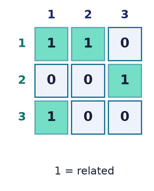
For the “strictly less than” relation on :
| 1 | 2 | 3 | 4 | |
|---|---|---|---|---|
| 1 | 0 | 1 | 1 | 1 |
| 2 | 0 | 0 | 1 | 1 |
| 3 | 0 | 0 | 0 | 1 |
| 4 | 0 | 0 | 0 | 0 |
The matrix form is ideal for checking structural properties by inspection and for computing compositions and closures (below). Its size is fixed at bits regardless of how many pairs are present, so it is best for dense relations.
3.5.3 As a directed graph (digraph)
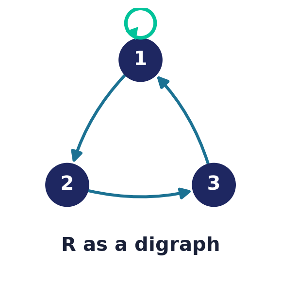
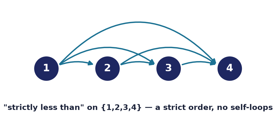
Draw one vertex (node) per element and one arrow for every pair . A pair becomes a self-loop at . For “strictly less than” on the digraph has four vertices with arrows from every smaller number to every larger one.
Two extreme relations are worth naming, both instantly recognisable in matrix form:
- Universal (full) relation — ; every pair is related, so the matrix is all ones.
- Empty relation — ; no pair is related, so the matrix is all zeros.
A third, quietly important, is the identity (diagonal) relation
also called the equality relation; its matrix is the identity matrix and its digraph is a self-loop at every vertex and nothing else. We will use constantly when defining reflexive closures and powers of a relation.
Remark (bridge to Lecture 10). A relation on a set is exactly the data of a directed graph, and a symmetric relation with no self-loops is exactly an undirected graph. The matrix is the graph’s adjacency matrix. Graph theory (Lecture 10) can therefore be read as the study of relations from a visual, combinatorial angle.
3.6 Properties of binary relations
Let be a relation on a set . The following properties classify how behaves; each has a crisp logical definition, a matrix “fingerprint”, and — as we prove in §3.6.1 — a slick algebraic form.
Definition 3.5. The relation on is
- reflexive if . Matrix: the whole main diagonal is .
- irreflexive if . Matrix: the whole diagonal is .
- symmetric if . Matrix: .
- antisymmetric if . Matrix: no off-diagonal mirror pair with .
- asymmetric if . Matrix: zero main diagonal and no mirror pair (equivalently ).
- transitive if . Matrix: wherever a two-step path exists, the direct entry is also .
- antitransitive if — a two-step path never has its direct shortcut. Example: the successor chain on ; or “beats” in rock–paper–scissors.
Common pitfall (reflexive vs. irreflexive are not opposites). A relation can be neither. On the relation has but not , so it is neither reflexive (misses ) nor irreflexive (has ). “Not reflexive” means some diagonal entry is missing; “irreflexive” means every diagonal entry is missing. Likewise symmetric and antisymmetric are not opposites: the identity relation is both, while is neither.
Proposition 3.6 (asymmetric irreflexive antisymmetric). is asymmetric iff is both irreflexive and antisymmetric.
Proof. () Suppose is asymmetric. Taking in the definition, , which forces for every ; hence is irreflexive. For antisymmetry, suppose and ; asymmetry applied to gives , contradicting . So the hypothesis is never satisfiable, and the implication “” holds vacuously. () Suppose is irreflexive and antisymmetric, and suppose . If also , antisymmetry gives , whence — contradicting irreflexivity. Therefore , and is asymmetric.
A strict order such as on is the archetypal asymmetric relation.
Worked example 3.7 (checking properties from a matrix). Consider on :
| 1 | 2 | 3 | 4 | |
|---|---|---|---|---|
| 1 | 0 | 0 | 1 | 1 |
| 2 | 1 | 0 | 1 | 1 |
| 3 | 0 | 0 | 0 | 0 |
| 4 | 0 | 0 | 0 | 0 |
So .
- Reflexive? No — the diagonal is all (in fact is irreflexive).
- Symmetric? No — but .
- Antisymmetric? Yes — there is no mirror pair with .
- Transitive? Yes — the only two-step chains start at : then needs ✓, and then needs ✓. Every other chain dies immediately because rows and are empty. Since all required “shortcuts” are present, is transitive.
Worked example 3.8 (a symmetric relation). The matrix
| 1 | 2 | 3 | 4 | |
|---|---|---|---|---|
| 1 | 0 | 1 | 1 | 0 |
| 2 | 1 | 0 | 0 | 0 |
| 3 | 1 | 0 | 0 | 0 |
| 4 | 0 | 0 | 0 | 0 |
satisfies , so is symmetric: every arrow is matched by , and in the digraph edges come in bidirectional pairs. It is not transitive: and but .
3.6.1 Algebraic characterisations
Each property can be phrased purely in the algebra of relations — using the identity relation , the inverse (§3.7) and composition . These forms are the ones that make later proofs short.
Theorem 3.9. For a relation on :
- is reflexive .
- is symmetric .
- is antisymmetric .
- is transitive (equivalently ).
Proof. (1) says for all , i.e. for all — the definition of reflexive.
(2) By definition . If is symmetric and then , so by symmetry ; hence . The reverse inclusion is symmetric (swap roles), giving . Conversely if and , then , so , i.e. ; thus is symmetric.
(3) Suppose is antisymmetric and . Then (so ) and (so , i.e. ); antisymmetry gives , so . Conversely, suppose and . Then and , so , whence .
(4) Suppose is transitive and . Then there is with and ; transitivity gives . Hence . Conversely suppose and . Then , so ; thus is transitive.
Remark. Part (4) is the engine behind transitive closure (§3.8): “make transitive” means “keep composing with itself until nothing new appears”.
3.6.2 Counting relations with a given property
Because a relation on an -element set is exactly a filling of an grid of bits, counting them is pure combinatorics — a favourite source of exam problems and a first taste of the counting techniques of later lectures.
Proposition 3.10. On a set with :
- the number of relations is ;
- the number of reflexive relations is ;
- the number of symmetric relations is ;
- the number of antisymmetric relations is .
Proof. Each of the cells is independently or , giving relations. For reflexive relations the diagonal cells are forced to and the remaining cells are free: . For symmetric relations the diagonal cells are free and the cells strictly above the diagonal are free, while each cell below the diagonal is forced to equal its mirror; this gives . For antisymmetric relations the diagonal cells are free ( choices), while each of the mirror-pairs with may be filled in exactly admissible ways — , , or (but not ) — giving .
Example 3.11. For : relations in all; reflexive; symmetric; antisymmetric; and relations that are both reflexive and symmetric (diagonal forced to , the three upper cells free).
3.7 Inverse and composition of relations
Definition 3.12 (inverse). The inverse (or converse) of is
so that . In matrix terms ; in the digraph, every arrow is reversed.
For instance the inverse of “less than” is “greater than”, and the inverse of “is a child of” is “is a parent of”. By Theorem 3.9(2), is symmetric exactly when .
Definition 3.12a (complement). The complement of a relation on a set is — the pairs omits — so that . In matrix terms every entry flips ; in the digraph, present and absent arrows swap. For example, the complement of is , and the complement of is .
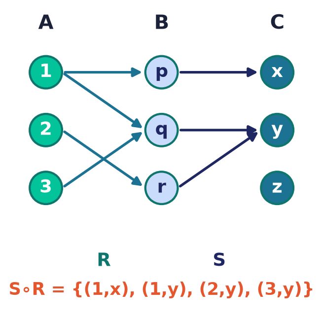
Definition 3.13 (composition). Given and , their composition is
Read right-to-left: “ first, then ”, exactly as with function composition . Composition chains relations through a common middle set.
Common pitfall (order matters, and it flips for matrices). In general ; they may even live in different Cartesian products. And note the reversal in the matrix formula below: the composite corresponds to the product , with the factors in the opposite order to the composition symbols.
Worked example 3.14. Let , , , with and . Tracing paths , , gives
3.7.1 Composition via the Boolean matrix product
The Boolean matrix product multiplies two matrices like ordinary matrices but with logical OR () in place of and logical AND () in place of . For an matrix and an matrix ,
Theorem 3.15 (composition = Boolean product). Let and with , , . Then
Proof. Write (so ) and (so ). Fix indices . By the definition of the Boolean product,
By the meaning of the matrix entries this says
which is precisely the defining condition for (Definition 3.13). Hence . As the two matrices agree in every entry, they are equal.
Worked example 3.16 (Example 3.14, done by matrix). Index , , :
Then
i.e. , reproducing the hand computation.
Remark (why OR, not ). A relation records only whether a connecting element exists, never how many. Using ordinary would count the number of intermediate ’s (e.g. give a ), which is meaningless for a relation. Replacing by (equivalently, capping every sum at ) keeps us inside and matches the existential quantifier “” in Definition 3.13.
3.7.2 Associativity, and powers of a relation
Theorem 3.17 (associativity of composition). For , , ,
Proof. Both sides are subsets of ; we show they contain the same pairs. For arbitrary ,
On the other side,
The two final conditions differ only in the order of the independent existential quantifiers versus ; since and range over unrelated sets, both simply assert the existence of a pair with the stated three-part property. Hence the conditions are logically equivalent, and the two sets coincide.
Associativity is exactly what lets us write powers of a relation on without brackets. Define
and, for reflexive/transitive purposes, . By Theorem 3.17, regardless of grouping, and by Theorem 3.15 the powers are computed by repeated Boolean matrix products: .
Lemma 3.18 (powers count paths). For , iff there exist with , , and for every — that is, iff there is a directed walk of length from to in the digraph of .
Proof. Induction on . Base : , and a walk of length from to is exactly a single edge . Step: assume the claim for . Then
By the induction hypothesis iff there is a walk of length ; appending the edge yields a walk of length . Conversely any length- walk from to splits at its penultimate vertex into a length- walk (so ) followed by the edge . Hence iff such a walk exists.
This “walks” reading is the key to understanding transitive closure, to which we now turn.
3.8 Closures of a relation
Sometimes a relation lacks a property we need. The closure of with respect to a property is the smallest relation that contains and has property — it adds as few pairs as possible. “Smallest” means: it is contained in every relation that contains and has . (When such a smallest relation exists it is automatically unique, since if were both smallest then and .)
3.8.1 Reflexive and symmetric closures
Definition/Theorem 3.19. Let be a relation on .
- The reflexive closure is .
- The symmetric closure is . Each is the smallest relation with the stated property containing .
Proof. Reflexive. , so it is reflexive (Theorem 3.9(1)), and . If is any reflexive relation with , then (reflexivity) and , hence . So is smallest.
Symmetric. First is symmetric: take . If then ; if then ; either way . Clearly . Now let be symmetric with . Then implies , and by symmetry (Theorem 3.9(2)), so . Hence , and is smallest.
3.8.2 Transitive closure and the connectivity relation
The transitive closure is subtler: adding shortcuts for existing two-step paths may create new two-step paths, which need their own shortcuts, and so on. The correct construction gathers all finite walks.
Definition 3.20. The transitive closure of is denoted or , and the reflexive–transitive closure (or connectivity relation) is .
Theorem 3.21 (transitive-closure formula). For any relation on a set ,
That is, is transitive, contains , and is contained in every transitive relation containing .
Proof. Write . We verify the three defining properties.
(i) . Immediate, since is one of the terms of the union.
(ii) is transitive. Suppose and . Then for some and for some . By Lemma 3.18 there is a walk of length from to and a walk of length from to ; concatenating them (the first ends where the second begins) yields a walk of length from to . By Lemma 3.18 again, . Hence is transitive.
(iii) Minimality. Let be any transitive relation with . We show for all by induction. Base: . Step: assume . Take ; then there is with and . By the induction hypothesis , and ; transitivity of gives . Thus . By induction for every , so .
By (i)–(iii), is a transitive relation containing and contained in every such relation; hence it is the smallest one, i.e. .
On an infinite set the union may be genuinely infinite (think of the successor relation on , whose transitive closure is ). On a finite set, however, the union stops early.
Theorem 3.22 (termination on a finite set). If , then
Proof. Since by Theorem 3.21, it suffices to prove that every with is already contained in ; the inclusion is clear. So suppose for some . Among all lengths for which , choose the minimum such ; by Lemma 3.18 there is a walk
We claim . Suppose not, so ; then the walk lists vertices , all drawn from the -element set . By the pigeonhole principle two of them coincide: for some . Excise the loop between positions and to obtain the shorter sequence
This is still a valid walk from to : the only new consecutive pair is , an original edge. Its length is , contradicting the minimality of . Therefore , so .
Remark (Warshall’s algorithm — a CS connection). Theorem 3.22 already gives an algorithm: compute by Boolean matrix products and OR them together, at a cost of bit-operations. Warshall’s algorithm (Stephen Warshall, 1962) computes far more cleverly in : it processes the vertices one at a time, after step recording exactly those pairs joined by a walk whose intermediate vertices all lie in , via the update “”. This is the Boolean specialisation of the Floyd–Warshall shortest-path algorithm and underlies reachability queries in graphs and databases.
Worked example 3.23 (all three closures). For on :
Worked example 3.24 (closure can become universal). Let be the directed -cycle on . Then
and contains all pairs: the transitive closure of a directed cycle through every vertex is the universal relation. (Note , so nothing new would ever appear — consistent with the bound of Theorem 3.22.)
3.9 Equivalence relations, classes and partitions
Definition 3.25 (equivalence relation). A relation on that is simultaneously reflexive, symmetric and transitive is an equivalence relation. We usually write it (or ) and read as “ is equivalent to ”.
Equivalence relations formalise “being the same for our present purposes”: having the same remainder on division by , the same colour, the same connected component, the same last digit, the same value under some measurement. They are the tool by which we deliberately forget irrelevant distinctions.
Definition 3.26 (equivalence class). For , the equivalence class of is — everything equivalent to . Any is called a representative of the class.
We also need the companion notion from Lecture 2.
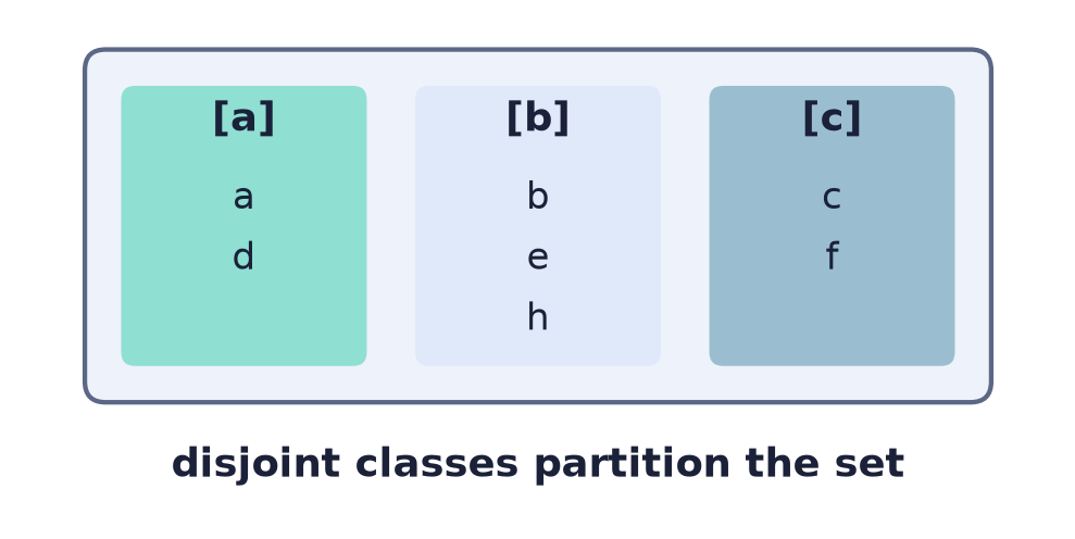
Definition 3.27 (partition). A partition of a set is a collection of subsets (the blocks or cells) of such that (i) every block is nonempty; (ii) distinct blocks are disjoint; and (iii) the blocks cover , i.e. .
3.9.1 The Fundamental Theorem of Equivalence Relations
We first isolate the two facts on which everything hinges.
Lemma 3.28. Let be an equivalence relation on . For all , .
Proof. () Suppose . We show : if then ; combined with , transitivity gives , so . By symmetry also gives , and the same argument yields . Hence . () Suppose . By reflexivity , so , which means .
Lemma 3.29 (classes are equal or disjoint). Let be an equivalence relation on . For all , either or .
Proof. Suppose the classes are not disjoint; we show they are equal. Pick . Then and . By symmetry , and with transitivity gives ; Lemma 3.28 then yields . So whenever the classes meet they coincide, which is exactly the stated dichotomy.
Theorem 3.30 (Fundamental Theorem of Equivalence Relations). Let be a nonempty set.
- If is an equivalence relation on , then the set of equivalence classes is a partition of .
- Conversely, if is a partition of , then the relation defined by
is an equivalence relation on , and its equivalence classes are exactly the blocks of . 3. The two constructions are mutually inverse: they set up a bijection between equivalence relations on and partitions of .
Proof of (1). We check the three conditions of Definition 3.27 for .
- Nonempty blocks. By reflexivity , so ; hence no class is empty.
- Cover. Each class , and every element lies in the class , so .
- Disjointness. Two distinct classes are disjoint by Lemma 3.29 (if they intersected they would be equal, not distinct).
Thus the distinct classes form a partition of .
Proof of (2). Write for . Because the blocks of cover and are pairwise disjoint, every lies in exactly one block; call it . Then by definition .
- Reflexive: , so .
- Symmetric: , so .
- Transitive: and give , so . Hence is an equivalence relation. Its class of is , the block containing . So the equivalence classes are precisely the blocks of .
Proof of (3). Start from an equivalence relation , form the partition , then form its “same-block” relation. Two elements share a block iff they lie in the same class, i.e. iff , iff (Lemma 3.28) ; so we recover . Conversely, start from a partition , form , then take its classes; by part (2) these are exactly the blocks of , so we recover . The two constructions are therefore inverse to each other, establishing the bijection.
Remark (why this matters). Theorem 3.30 says that “equivalence relation” and “partition” are two languages for the same phenomenon. Whenever you sort objects into non-overlapping categories that between them cover everything, you have — like it or not — defined an equivalence relation, and vice versa. This is why the theorem is invoked all over mathematics and CS: connected components of a graph, congruence classes of integers, types in a type system, disjoint-set (union–find) data structures, and — in Lecture 13 — the decomposition of a sample space into mutually exclusive, exhaustive events on which probabilities are summed.
The set of classes is called the quotient set of by , and (equivalently, the number of equivalence relations on it) is the Bell number; .
Worked example 3.31 (three views of one equivalence relation). On define (“congruent modulo ”). It is reflexive (), symmetric () and transitive (if and then ), hence an equivalence relation. Its classes are
giving the partition of . Conversely, starting from this partition and declaring two numbers equivalent when they share a block returns exactly — the round trip promised by Theorem 3.30(3).
3.9.2 Application: congruence classes and modular arithmetic
Fix an integer . On the whole set define
Theorem 3.32. Congruence modulo is an equivalence relation on with exactly classes, namely the residue classes , where .
Proof. Reflexive: . Symmetric: if then , so . Transitive: if and then , so . Hence is an equivalence relation. By the division algorithm every integer can be written with a unique remainder ; then , so and . Thus the classes cover . They are distinct because if then , so and . Hence there are exactly classes.
The quotient set is written . The reason it is genuinely useful is that arithmetic descends to the classes:
Theorem 3.33 (arithmetic is well-defined mod ). If and , then and .
Proof. Write and for integers . Then
so , i.e. . And
so , i.e. .
Consequently the definitions and do not depend on which representatives we pick — the operations are well-defined on , turning it into a finite arithmetic system.
Common pitfall (well-definedness is not automatic). Not every formula on representatives descends to classes. On the “operation” is ill-defined: but while , so the answer depends on the representative. Theorem 3.33 is a genuine theorem, not a triviality, precisely because such failures are possible.
CS connections. Modular arithmetic is the arithmetic of finite machines and is everywhere in computing: hash functions and hash tables (), checksums and cyclic redundancy checks, pseudo-random generators, cyclic buffers (indices mod capacity), clock arithmetic, and the public-key cryptosystem RSA, whose security rests on modular exponentiation. All of these silently rely on the fact that congruence classes form a well-behaved arithmetic (Theorems 3.32–3.33).
3.10 Partial orders, Hasse diagrams, and a first look at lattices
Definition 3.34 (partial order, poset). A relation on that is reflexive, antisymmetric and transitive is a partial order. The pair is a partially ordered set (poset). We write for “ and ” (the associated strict order).
Partial orders model ranking with possible incomparabilities: precedence of tasks, refinement of specifications, subset containment, divisibility, information order. Compare with equivalence relations: swap symmetry for antisymmetry and the character changes completely — from “grouping equals” to “ordering unequals”.
3.10.1 Comparability and total orders
Definition 3.35. In a poset , elements are comparable if or ; otherwise they are incomparable (written ). If every pair is comparable, is a total (or linear) order, and is a chain.
Examples: on , or is total; alphabetical/lexicographic order on strings is total; but subset order and divisibility are only partial.
Worked example 3.36 (divisibility is a partial order). Divisibility on (the positive divisors of ) is a partial order: (reflexive); for positive integers and force (antisymmetric); and , give (transitive). It is only partial: and both fail, so ; likewise .
3.10.2 Hasse diagrams
Drawing every arrow of a partial order is wasteful: reflexive loops and transitivity-forced edges clutter the picture. A Hasse diagram strips it to essentials.
Definition 3.37 (cover; Hasse diagram). In a poset, covers (written ) if and there is no with . The Hasse diagram draws one node per element and one line for each covering pair, placing the smaller element lower; direction is read off the vertical position, so no arrowheads are needed. Reflexive loops and transitively implied edges are omitted.
Worked example 3.38 (Hasse diagram of ). For the covering pairs are
(e.g. is not a cover because , and is not a cover because ). An ASCII sketch (with at the bottom and at the top):
            12
           /  \
          4    6
          |   / \
          2 -/   3
          |     /
          1 ---/
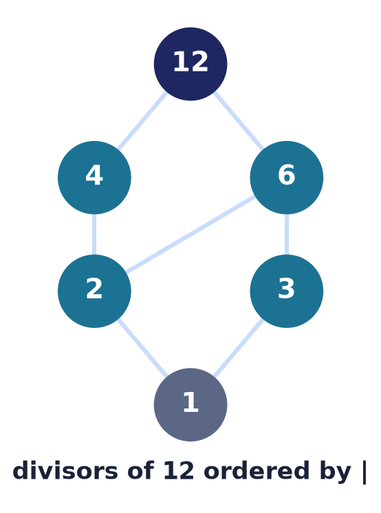
Here the seven line-segments realise the seven covers above: sits over and ; over ; over both and ; and under both and . All other relationships (such as or ) are recovered by following lines upward and using transitivity.
3.10.3 Minimal, maximal, least and greatest elements
Let be a poset and .
Definition 3.39.
- is a minimal element of if no satisfies (nothing in lies strictly below ).
- is a maximal element of if no satisfies .
- is the least (or minimum) element if for every .
- is the greatest (or maximum) element if for every .
Common pitfall (minimal least). Minimal means “nothing below it”; least means “below everything”. A poset may have several minimal elements and no least element. In the whole set has least element and greatest element ; but the subset has two minimal elements ( and ) and no least element, and two maximal elements ( and ) with no greatest.
Theorem 3.40 (uniqueness). A subset of a poset has at most one least element and at most one greatest element.
Proof. Suppose are both least elements of . Since is least and , . Since is least and , . Antisymmetry gives . The greatest-element case is dual (reverse every ).
Because of Theorem 3.40 we may speak of the least element and the greatest element when they exist.
Theorem 3.41 (least unique minimal). If has a least element , then is the unique minimal element of .
Proof. First, is minimal: if and , then (as is least), so antisymmetry gives ; hence no element is strictly below . Now let be any minimal element of . Since is least, . If then with , contradicting the minimality of . Therefore , so is the only minimal element.
Theorem 3.42 (finite posets have extremal elements). Every finite nonempty poset has at least one minimal element and at least one maximal element.
Proof (minimal; maximal is dual). Note is irreflexive ( would require ). Pick any . If is minimal, stop. Otherwise choose ; if is minimal, stop; otherwise choose , and so on, generating . These elements are pairwise distinct: if with , then chaining the strict steps by transitivity gives , i.e. , impossible. Since is finite the process cannot continue forever, so it must halt — and it halts only when it reaches a minimal element.
Remark (why finiteness is needed). In an infinite poset a unique minimal element need not be least. Let , where the negative integers carry their usual order (descending forever, with no minimum) and is a brand-new element declared incomparable to every negative integer. No negative integer is minimal (each has a smaller one below it), while is minimal (nothing is below it), so is the unique minimal element. Yet is not least: . Theorem 3.42 fails here precisely because the descending chain never terminates.
3.10.4 Bounds and a first look at lattices
Beyond elements of , we often care about elements of the whole poset that sit above or below all of .
Definition 3.43. Let in a poset . An element is an upper bound of if for all ; a lower bound satisfies for all . The least upper bound (supremum, join), if it exists, is the least element of the set of upper bounds, written ; for two elements it is . Dually the greatest lower bound (infimum, meet) is , written .
By Theorem 3.40, joins and meets are unique when they exist.
Definition 3.44 (lattice). A poset is a lattice if every pair of elements has both a join and a meet .
Example 3.45 (three familiar lattices).
-
Power set : here and (Lecture 2’s operations are literally join and meet). Its Hasse diagram for is the diamond
{a,b} / \ {a} {b} \ / ∅ -
Divisibility : and . The poset of Example 3.38 is a finite lattice; e.g. and .
-
Total orders are lattices with and .
Example 3.46 (a poset that is not a lattice). Take with and , (a “crown”). ASCII (the two middle segments cross at ):
      c     d
      | \ / |
      |  ×  |
      | / \ |
      a     b
The pair has upper bounds and , but , so there is no least upper bound; does not exist and is not a lattice. (Dually, has no meet.)
Remark (forward pointer). A lattice that is also bounded (has a least element and greatest element ), distributive, and complemented is a Boolean algebra — the algebraic skeleton of propositional logic and digital circuits. The power-set lattice is the prototype. We return to Boolean algebra in a later lecture; for now, note how the set operations of Lecture 2 already exhibit the lattice structure in miniature.
3.11 -ary relations and the relational database model
Definition 3.47 (-ary relation). An -ary relation is a subset ; its elements are -tuples. Binary relations are the case , and the Cartesian product itself is the universal -ary relation.
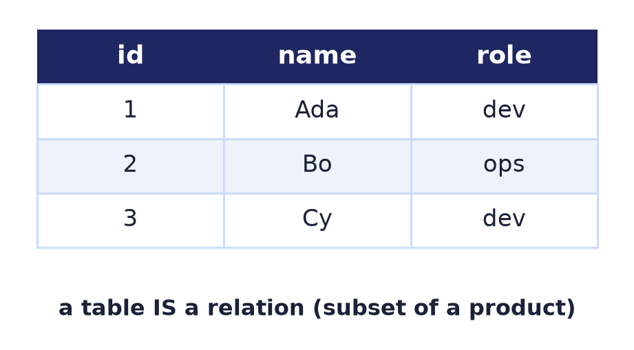
Motivating example (students · subjects · marks). Let
An examination record is a ternary relation , e.g.
This is exactly a database table: each tuple is a row (record), each factor is a column (attribute) with its own domain, and is the number of columns (the table’s arity).
| STUDENT | SUBJECT | MARK |
|---|---|---|
| Shevchenko | Programming | B |
| Kosach | Algebra | A |
| Franko | Discrete Math | E |
Remark (a set has no duplicates and no order). Because a relation is a set of tuples, a table in this idealised model has no duplicate rows and no inherent row order — mirroring the mathematical fact that and that sets are unordered. Real SQL tables relax this (bags, not sets), but the theory is set-based.
3.11.1 Relational algebra
Since relations are sets, the operations of Lecture 2 apply between two relations of the same shape (same sequence of attribute domains): union , intersection , and difference . Adding a few relation-specific operators yields relational algebra, the theory underlying SQL, introduced by E. F. Codd in 1970.
- Selection — keep the rows (tuples) satisfying a
condition ; chooses a subset of the tuples. (SQL
WHERE.) - Projection — keep only certain columns, discarding
the others (and any duplicate rows that result); chooses a subset of the
attributes. (SQL
SELECTof specific columns.) - Cartesian product — pair every row of with every row of (the same product as in §3.2).
- Natural join — combine rows of and that agree on their shared attribute(s); a filtered, matched Cartesian product. It is the workhorse that reconnects data split across tables.
Worked example 3.48 (projection, selection, join). Let
| ENROLL: STUDENT | COURSE |
|---|---|
| Kosach | Algebra |
| Kosach | DM |
| Franko | DM |
and
| OFFER: COURSE | ROOM |
|---|---|
| Algebra | 101 |
| DM | 205 |
Then (the duplicate Kosach collapses); keeps the two DM rows; and the natural join on COURSE is
| ENROLL ⋈ OFFER: STUDENT | COURSE | ROOM |
|---|---|---|
| Kosach | Algebra | 101 |
| Kosach | DM | 205 |
| Franko | DM | 205 |
each enrolment matched to the room where its course is offered.
So the abstract notion of an -ary relation is not merely theory: it is the data model every relational database implements, and the humble set operations of Lecture 2 are its computational core.
3.12 Functions as a special kind of relation
Definition 3.49 (functional relation; function). A relation is functional (single-valued) if each relates to at most one : whenever and , then . If in addition every relates to exactly one , then is a total function , and we write in place of .
Thus a function is a relation — one obeying the single-valuedness condition. Its domain is its set of inputs and its range is the set of attained outputs — the very domain/range of §3.4. Functions may be injective (distinct inputs give distinct outputs), surjective (every element of is attained), or bijective (both) — the properties we have just defined, which recur throughout the course (for example in counting and in graph isomorphism).
Common pitfall (which relations fail to be functions). On the relation is not a function: the input has two outputs, so single-valuedness fails. The relation is a (partial) function even though two inputs share the output — single-valuedness restricts outputs per input, not inputs per output. And a total function additionally forbids the input from having no output at all.
Remark. Reading a function as its graph is not a mere formality: it is how functions are defined rigorously in set theory, and how they are stored (as key–value tables) in computing.
Historical note
The set-theoretic viewpoint on relations grew out of Georg Cantor’s creation of set theory in the 1870s–1880s. The now-standard encoding of the ordered pair, , is due to Kazimierz Kuratowski (1921) and is what lets relations be defined purely as sets (Lecture 2). Modular arithmetic — our flagship equivalence relation — was placed on a firm footing by Carl Friedrich Gauss in the Disquisitiones Arithmeticae (1801), which introduced the congruence notation . The systematic theory of order and lattices was developed by Richard Dedekind around 1900 (his Dualgruppen) and brought to maturity by Garrett Birkhoff, whose Lattice Theory (1940) is the classic reference; the diagrams are named after Helmut Hasse. The transitive-closure algorithm of §3.8 is due to Stephen Warshall (1962). Finally, the entire -ary story found its most consequential application when Edgar F. (“Ted”) Codd of IBM published A Relational Model of Data for Large Shared Data Banks (Communications of the ACM, 1970), founding the relational database — arguably the single most commercially important application of discrete mathematics.
Chapter summary
- A relation is a subset of a Cartesian product; a binary relation is , with written . Specify it by listing or by a predicate; represent it as a set of pairs, a Boolean matrix, or a digraph. The identity relation and the universal/empty relations are the reference points.
- Domain and range collect the first and second components that occur.
- Core properties — reflexive, irreflexive, symmetric, antisymmetric, asymmetric, transitive (and the rarer antitransitive) — each have a matrix fingerprint and an algebraic form: ; ; ; (Theorem 3.9). Counting relations with a property is combinatorics (Proposition 3.10).
- Inverse transposes the matrix / reverses arrows. Composition chains relations and equals the Boolean matrix product (Theorem 3.15); composition is associative (Theorem 3.17), so powers are well-defined and count walks of length (Lemma 3.18).
- Closures add the fewest pairs to gain a property: , , and (Theorem 3.21), a finite union on an -element set (Theorem 3.22, via pigeonhole); Warshall’s algorithm computes it in .
- Equivalence relations (reflexive + symmetric + transitive) correspond exactly to partitions via the Fundamental Theorem (Theorem 3.30), proved in both directions. The prototype is congruence mod , whose classes support well-defined modular arithmetic (Theorems 3.32–3.33).
- Partial orders (reflexive + antisymmetric + transitive) are drawn as Hasse diagrams. Distinguish minimal/maximal from least/greatest: least/greatest are unique when they exist (Theorem 3.40) and finite posets always have extremal elements (Theorem 3.42). Adding joins and meets for every pair gives a lattice; power sets and divisibility are the standard examples.
- -ary relations are precisely the tables of the relational database model, manipulated by relational algebra (selection, projection, product, natural join). A function is the special case of a single-valued relation.
Exercises
Warm-up
W1. Let and . (a) Write the relation matrix. (b) Give and . (c) Decide whether is reflexive, symmetric, antisymmetric, transitive.
W2. For the of W1, compute as a set of pairs and give its matrix. How is related to ?
W3. On let and . Compute and . Are they equal?
W4. For each relation on decide which of reflexive / symmetric / antisymmetric / transitive it has: (a) ; (b) ; (c) .
W5. List the equivalence classes of congruence modulo on , and write the induced partition.
W6. For on give the reflexive closure and the symmetric closure .
Standard
S7. Let on . Compute and hence . Is the universal relation? Explain using Theorem 3.22 why you need not compute beyond .
S8. On define and have the same parity (both even or both odd). Prove is an equivalence relation and describe its classes as a partition of .
S9. Consider divisibility on . (a) State why it is a poset. (b) List all covering pairs and describe the Hasse diagram. (c) Identify the least, greatest, minimal and maximal elements. (d) Is a lattice? Compute and .
S10. On an -element set, count (a) all relations, (b) reflexive relations, (c) symmetric relations, (d) relations that are both reflexive and symmetric. Evaluate each for .
S11. Let on . Use the Boolean matrix product to compute and list . Is transitive? Justify via Theorem 3.9(4).
S12. Prove that if and are transitive relations on , then is transitive. Then give a concrete example on of two transitive relations whose union is not transitive.
S13. The partition of induces an equivalence relation . List all pairs of and state .
S14. With ENROLL and OFFER as in Example 3.48, write out (a) , (b) , and (c) the natural join , explaining in one sentence what each result represents.
Challenge
C15. Prove that composition distributes over union: for relations of compatible shapes. Show also that , and give an example where the inclusion is strict.
C16 (equivalence closure). (a) Prove that the intersection of any nonempty family of equivalence relations on is again an equivalence relation. (b) Deduce that for any relation on there is a smallest equivalence relation containing . (c) Prove that .
C17. Let be a poset. (a) Prove that if is finite and nonempty then it has a maximal element. (b) Prove that if a finite poset has a unique maximal element, that element is the greatest. (c) Give an infinite poset with a unique maximal element that is not greatest.
C18. (a) Prove that the number of symmetric relations on an -set is and the number of antisymmetric relations is . (b) How many relations are both symmetric and antisymmetric? Identify them explicitly. (c) Explain why the count of equivalence relations is the Bell number , and compute .
Selected answers & hints
W1. (a) Rows/cols indexed :
| 1 | 2 | 3 | 4 | |
|---|---|---|---|---|
| 1 | 1 | 1 | 0 | 0 |
| 2 | 0 | 0 | 1 | 0 |
| 3 | 0 | 0 | 0 | 1 |
| 4 | 0 | 0 | 0 | 1 |
(b) , . (c) Not reflexive (); not symmetric (, ); antisymmetric (no off-diagonal mirror pair); not transitive ( but ).
W3. (“ then ”): gives ; gives ; gives . So . (“ then ”): , , give . They are not equal — composition is not commutative.
W5. , , , ; partition .
S7. , , . Their union with is all pairs, so , the universal relation. Since , Theorem 3.22 guarantees , so no higher power is needed (indeed ).
S8. Reflexive: has the same parity as itself. Symmetric: if share parity then so do . Transitive: if share parity and share parity, then share parity (parity is a two-valued attribute). Classes: the evens and the odds ; partition . (This is congruence mod , a special case of Theorem 3.32.)
S10. (a) ; (b) ; (c) ; (d) . For : respectively.
S12. If then both pairs lie in (so by transitivity of ) and both lie in (so ); hence . Counterexample for union: and are each transitive (no composable pairs within either), but lacks and is not transitive.
C16. Hints. (a) Reflexivity: each , so . Symmetry and transitivity: if a pair (or two composable pairs) lie in the intersection, they lie in every , which is symmetric/transitive, so the required consequence lies in every , hence in the intersection. (b) Apply (a) to the family of all equivalence relations containing (nonempty, since is one); their intersection is the smallest such, namely . (c) Show is an equivalence relation containing (reflexive since it, symmetric because is symmetric and transitive closure preserves symmetry, transitive by construction), so ; conversely any equivalence relation contains (symmetry), (reflexivity) and all their walks (transitivity), so , giving .
C17. Hints. (a) Mirror Theorem 3.42 with ascending chains. (b) In a finite poset every element lies below some maximal element (ascend a chain until it stops); if the maximal element is unique, every element lies below it, so it is greatest. (c) Take with the usual order on the positive integers (ascending forever, no maximum) and incomparable to all of them: is the unique maximal element but , so is not greatest.
Further reading
- Kenneth H. Rosen, Discrete Mathematics and Its Applications, 8th ed., Chapter 9 (“Relations”): §9.1 relations and their properties, §9.3 representing relations, §9.4 closures (Warshall’s algorithm), §9.5 equivalence relations, §9.6 partial orderings and lattices.
- Susanna S. Epp, Discrete Mathematics with Applications, 5th ed., Chapter 8 (“Relations”): reflexivity/symmetry/transitivity, equivalence relations and partitions, partial-order relations.
- E. F. Codd, “A Relational Model of Data for Large Shared Data Banks”, Communications of the ACM 13(6), 1970 — the origin of the relational database connection in §3.11.
- (For the order-theory strand) Garrett Birkhoff, Lattice Theory, American Mathematical Society — the classic reference behind §3.10.4.