Lecture 11. Graph theory — algorithms
11.1 Overview
Lecture 10 developed the static language of graphs: vertices and edges, degrees, adjacency representations, weighted graphs, and the two coloring invariants — the chromatic number (fewest colors for a proper vertex coloring) and the chromatic index (fewest colors for a proper edge coloring). That lecture told us what these quantities are; it did not tell us how to compute anything. This lecture is about doing things with graphs: first the two systematic traversals (breadth- and depth-first search) that visit every vertex, then five classical algorithms that produce colorings, shortest paths, and cheapest connecting networks, together with the data structures that make them fast and the proofs that make them trustworthy.
Three questions organize the chapter, each drawn from a real computational need.
- How do we schedule conflicting tasks with as few resources as possible? This is graph coloring. We study greedy vertex coloring and greedy edge coloring — fast, simple heuristics that always produce a valid coloring and come with provable upper bounds on how many colors they use.
- What is the cheapest way to get from one place to every other place? This is the single-source shortest-path problem, solved by Dijkstra’s algorithm when edge weights are non-negative.
- What is the cheapest network that keeps everything connected? This is the minimum spanning tree problem, solved by Prim’s and Kruskal’s algorithms — two greedy routes to the same optimum, both justified by a single beautiful lemma, the cut property.
A recurring theme: greed
Every optimization algorithm in this lecture is greedy (the two traversals, BFS and DFS, are the exception): it builds its answer incrementally and, at each step, commits to the choice that looks best right now, never reconsidering. Greedy algorithms are attractive because they are simple and fast, but the deep question is always the same:
Does taking the locally best choice at every step lead to a globally optimal result?
The answer here is instructive precisely because it is not uniform:
- For shortest paths and minimum spanning trees, greedy is exactly optimal, and we will prove it — via the “finalized-distance” invariant for Dijkstra and via the cut property for Prim and Kruskal.
- For coloring, greedy is only an approximation: it always yields a proper coloring, but may use more colors than the optimum or , and the number it uses depends on the order in which objects are processed.
Keeping this contrast in mind — when greed is provably safe and when it is merely a bounded heuristic — is one of the main takeaways of the lecture.
Prerequisites and notation
We lean on the following from Lecture 10 (graph basics):
- A weighted graph attaches a real number — a weight, cost, length, or capacity — to each edge.
- The adjacency list stores, for each vertex , the list of its neighbors together with edge weights. It uses space and lets us scan a vertex’s incident edges in time proportional to its degree. This is the representation assumed throughout. The alternative adjacency matrix costs space and is only competitive on very dense graphs.
- A proper coloring never gives the same color to two adjacent objects (adjacent vertices for vertex coloring; edges sharing an endpoint for edge coloring).
- denotes the maximum degree of the graph, and the degree of vertex . Recall the Handshaking Lemma .
We write for the number of vertices and for the number of edges. Inside asymptotic bounds we follow the standard convention (as in CLRS) of writing and for these counts, so that “” means “”; the letters name the sets, but in an they stand for the sizes. Spanning trees, forests, and the structural theory of trees are the subject of Lecture 12; we borrow two facts from there and flag them where used.
The running graph — defined and drawn in the next section — places at the far left, at the far right, and / as two middle columns, with every edge labelled by its weight. The single figure is reused for all five algorithms: coloring ignores the weights, the path/tree algorithms use them.
11.2 A word on greedy algorithms
Before the graph algorithms, it helps to name the pattern they share.
Greedy algorithm — an algorithm that constructs a solution in a sequence of steps, and at each step irrevocably makes the choice that is locally optimal according to some fixed rule, without backtracking.
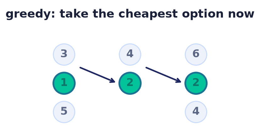
Two ingredients decide whether a greedy algorithm is correct (produces a globally optimal answer), rather than merely fast:
- The greedy-choice property: there is always a globally optimal solution that is consistent with the greedy first choice. (For MSTs this is exactly the cut property.)
- Optimal substructure: an optimal solution to the whole problem contains optimal solutions to subproblems, so that after making the greedy choice, solving the rest greedily still yields the optimum.
When both hold, an exchange argument (swap the greedy choice into an arbitrary optimal solution without making it worse) proves optimality. Shortest paths and MSTs enjoy both, which is why Dijkstra, Prim, and Kruskal are exact. Coloring lacks the greedy-choice property — the locally cheapest color can paint us into a corner — so greedy coloring is only a bounded approximation. (The deepest reason MST greed works is that the sets of “edges extendable to a spanning tree” form a matroid; matroids are exactly the structures on which greedy is always optimal. See Further reading.)
Remark. “Greedy” is a strategy, not a guarantee. The same word covers a provably optimal algorithm (Dijkstra) and a heuristic that can be arbitrarily far from optimal (greedy coloring on a bad ordering). Always ask which case you are in.
11.3 The running weighted graph
To let the results be compared, we run Dijkstra, Prim, and Kruskal — and, ignoring the weights, both coloring algorithms — on one shared weighted graph .
with the nine weighted edges
| Edge | Edge | Edge | |||
|---|---|---|---|---|---|
| 4 | 5 | 3 | |||
| 2 | 8 | 6 | |||
| 1 | 10 | 7 |
As adjacency lists (neighbors with weights):
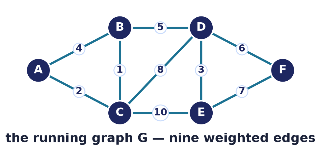
Degrees are , so the maximum degree is and (Handshaking check) . The graph is connected (needed for the MST algorithms) and its nine weights are distinct (which, as we prove later, makes the MST unique — so Prim and Kruskal must return the very same edge set, an ideal setup for comparison). It also contains several triangles (, , , ), which will force at least three colors.
11.4 Graph traversal: breadth-first and depth-first search
Before optimizing over a graph we must be able to visit it systematically — reach every vertex, discover the connected component of a start vertex, and build a tree of first-discoveries. The two canonical traversals differ only in the data structure that holds the frontier of discovered-but-unexplored vertices: a queue gives breadth-first search (BFS), a stack (or recursion) gives depth-first search (DFS).
BFS(G, s):                              DFS(G, s):          # recursive
    mark every vertex unvisited             mark s visited
    Q ← queue holding s;  visit s           for each neighbor w of s:
    while Q not empty:                          if w unvisited:
        u ← dequeue(Q)                              DFS(G, w)
        for each neighbor w of u:
            if w unvisited:
                visit w;  enqueue(Q, w)
DFS is usually written recursively — the call stack is the stack; an explicit-stack variant simply replaces BFS’s queue by a stack. Each vertex is enqueued once and each edge examined a constant number of times, so with adjacency lists both run in — linear in the size of the graph.
Worked trace on (weights ignored), starting at , neighbors in alphabetical order.
- BFS visits in rings of increasing distance from . Its tree of discovery edges is , and the ring number is exactly the fewest-edges distance from : .
- DFS plunges , backtracking only at dead ends; its discovery tree is the path .
Same vertices, different trees — BFS stays shallow and wide, DFS goes deep.
What traversal is for.
- Connectivity and components. One traversal reaches exactly the start vertex’s component; restarting from any still-unvisited vertex counts the connected components (§10.9) in .
- Shortest paths in an unweighted graph. BFS’s ring number is the minimum number of edges from the source — the unweighted counterpart of Dijkstra below, and far cheaper when the weights are all equal.
- Paths and cycles. DFS underlies path-finding, cycle detection, and topological
ordering; the
findPath/findCircuitroutines of Lab 6 are DFS at heart.
Traversal is the workhorse the rest of this chapter leans on: Dijkstra’s and Prim’s frontier-growing loops are BFS with a priority queue in place of a plain one.
11.5 Greedy vertex coloring
Motivation
Vertex coloring is the abstract form of conflict scheduling. Model each task as a vertex and join two tasks by an edge when they conflict (cannot share a resource). A proper coloring is then an assignment of resources — exam time slots, radio frequencies, CPU registers — such that no two conflicting tasks collide, and the number of colors is the number of resources needed. The classic compiler application is register allocation: variables are vertices, an edge means two variables are “live” simultaneously, colors are machine registers.
Finding exactly is NP-hard, so in practice we reach for a fast heuristic. The simplest is greedy.
The algorithm
Greedy vertex coloring — fix an ordering of the vertices; visit them in that order and give each vertex the smallest color (a positive integer ) not already used by any of its already-colored neighbors.
function GreedyVertexColoring(G, ordering v1..vn):
    for i = 1 to n:
        used ← { color[u] : u is a neighbor of vi and u already colored }
        color[vi] ← smallest positive integer not in used
    return color
Finding the smallest free color efficiently. Naively “scanning for a gap” sounds like
it could be slow, but it is not. Keep a scratch boolean array seen[1..Δ+1]. When coloring
, for each already-colored neighbor with set
seen[color[u]] ← true; then scan for the first index with
seen[c] = false. Because has at most colored neighbors, the answer is
at most , so the scan stops within steps. Reset only the entries
you touched (or use a version-stamp trick) so the per-vertex cost stays .
Worked trace
Run greedy on (ignoring weights) in the natural order . The “colored neighbors” column lists each neighbor that is already colored and its color.
| Step | Vertex | Colored neighbors (colors) | Forbidden colors | Assigned |
|---|---|---|---|---|
| 1 | — | 1 | ||
| 2 | 2 | |||
| 3 | 3 | |||
| 4 | 1 | |||
| 5 | 2 | |||
| 6 | 3 |
Colors used: — three colors. The final coloring is ; a quick check of all nine edges confirms every edge joins two differently colored endpoints, so it is proper.
Is three optimal? Yes: the triangle has three mutually adjacent vertices, all of which need distinct colors, so ; and greedy exhibited a proper -coloring, so and here greedy is optimal.
Correctness: greedy always produces a proper coloring
Theorem 11.1. For every graph and every vertex ordering, GreedyVertexColoring
returns a proper coloring.
Proof. Take any edge ; we must show .
Without loss of generality is colored before (one of them is). At the moment is
colored, is an already-colored neighbor of , so lies in the set
used that avoids. Hence . As was arbitrary,
no edge is monochromatic.
Correctness: the bound
Theorem 11.2. GreedyVertexColoring uses at most colors, for every ordering.
Consequently .
Proof. When vertex is colored, the forbidden set used is contained in the set of
colors of ’s already-colored neighbors, so .
Among the colors at most are forbidden, so at
least one is free; greedy picks the smallest free color, which is therefore .
No vertex ever receives a color exceeding , so the total number of colors used is
. Since the coloring is proper (Theorem 11.1), .
On , , so the theorem promises colors; greedy did much better with because the ordering was favorable.
Remark (Brooks’ theorem). The bound is rarely tight. Brooks’ theorem (1941) states that a connected graph satisfies unless is a complete graph (which needs ) or an odd cycle (which needs ). Our is neither, and indeed .
The ordering matters
Theorem 11.2 bounds the worst case, but the actual number of colors depends heavily on the processing order. Greedy is always proper, yet the color count is not.
A concrete gap on . Run greedy on the same graph in the order :
| Step | Vertex | Colored neighbors (colors) | Assigned |
|---|---|---|---|
| 1 | — | 1 | |
| 2 | — (none of colored yet) | 1 | |
| 3 | 2 | ||
| 4 | 3 | ||
| 5 | 4 | ||
| 6 | 2 |
This uses four colors, although . The culprit is vertex : by the time it is reached, its four neighbors already carry three distinct colors , forcing a fourth. Same graph, same algorithm, different order — one extra color.
A dramatic gap: the crown graph. The crown graph is with a perfect matching deleted: parts and , with adjacent to every except . It is bipartite, so . But process the vertices in the paired order : an easy induction shows and each see exactly the colors on already-colored neighbors and so receive color . Greedy therefore uses colors on vertices — arbitrarily far from the true value . (For this already forces colors instead of .) There is always an ordering achieving the optimum — color the vertices in the order an optimal coloring would — but finding such an order is as hard as coloring itself.
The Welsh–Powell heuristic
Since order is everything, a good default is to color high-degree vertices first, on the intuition that they are the hardest to satisfy and should be handled while colors are plentiful.
Welsh–Powell coloring — sort the vertices in non-increasing order of degree, then run greedy in that order.
function WelshPowell(G):
    sort vertices so that deg(v1) ≥ deg(v2) ≥ … ≥ deg(vn)
    return GreedyVertexColoring(G, v1..vn)
On the degrees are , giving the order :
| Step | Vertex | Colored neighbors (colors) | Assigned |
|---|---|---|---|
| 1 | — | 1 | |
| 2 | 2 | ||
| 3 | 3 | ||
| 4 | 3 | ||
| 5 | 2 | ||
| 6 | 1 |
Three colors — optimal. Welsh–Powell also yields the useful bound , where is the sorted degree sequence and is the position. It is a heuristic, not a guarantee: there exist graphs where even largest-degree-first is suboptimal. But it is cheap and usually good.
Complexity and data structures
Data structure: adjacency lists plus one reusable scratch array seen[1..Δ+1].
Time: for each vertex we do work (mark neighbor colors, scan for the first gap, reset). Summing over all vertices and using the Handshaking Lemma,
Welsh–Powell adds an sort, giving . Space is beyond the graph itself.
Common pitfall. Do not believe that greedy computes . It computes a proper coloring whose size is between and , and which depends on the ordering. If you need the true chromatic number you must search (exponential in the worst case).
CS connection. Chaitin’s classic register allocator (1981) models allocation as vertex coloring of an interference graph and colors it greedily; when more than colors (= registers) are needed, some variable is “spilled” to memory — the practical response to greedy’s non-optimality.
11.6 Greedy edge coloring
Motivation
Edge coloring is the natural model for timetabling round-robin schedules. Represent players (or teams, machines, people) as vertices and each required match/meeting as an edge; a color is a time slot. Two edges sharing an endpoint must get different colors (a player cannot play two matches at once), so a proper edge coloring is a conflict-free schedule and is the fewest time slots needed.
The algorithm
Greedy edge coloring — fix an ordering of the edges; give each edge the smallest color not used by any adjacent edge (an edge that shares an endpoint) that is already colored.
function GreedyEdgeColoring(G, ordering e1..em):
    for k = 1 to m:
        let ek = (u, v)
        used ← { color[e] : e already colored and e shares endpoint u or v with ek }
        color[ek] ← smallest positive integer not in used
    return color
This is literally greedy vertex coloring run on the line graph , whose vertices are the edges of and whose edges join pairs of -edges that share an endpoint. Every theorem about greedy vertex coloring transfers, with in place of .
Worked trace
Color processing edges in the order . Recall .
| Step | Edge | Adjacent colored edges (colors) | Assigned |
|---|---|---|---|
| 1 | — | 1 | |
| 2 | 2 | ||
| 3 | 3 | ||
| 4 | 2 | ||
| 5 | 1 | ||
| 6 | 4 | ||
| 7 | 3 | ||
| 8 | 4 | ||
| 9 | 1 |
Four colors. The four color classes are
and each is a matching (no two of its edges share a vertex; the formal treatment and Hall’s theorem are in Lecture 12 §12.9) — which is exactly what “proper edge coloring” means. Class is even a perfect matching, pairing up all six vertices. Since (the four edges at must all differ), greedy’s four colors are optimal here: .
Correctness and bounds
Theorem 11.3 (proper). GreedyEdgeColoring always returns a proper edge coloring.
Proof. It is Theorem 11.1 applied to the line graph : two edges sharing an endpoint
are adjacent vertices of , and the algorithm gives them different colors by the same
argument.
Theorem 11.4 (the bound). GreedyEdgeColoring uses at most
colors. Proof. An edge is adjacent to at most
other edges, hence to at most already-colored ones. Among the colors
at least one is free, and greedy takes the smallest such.
How good is ? Compare it with the optimum, pinned down by a famous theorem from Lecture 10.
Vizing’s theorem. Every simple graph satisfies .
So the true optimum is one of just two values, whereas greedy only promises — off by nearly a factor of two in the worst case. On greedy happened to hit the optimum , but in general greedy edge coloring is a weaker approximation than the theory allows.
Complexity
Data structure: adjacency lists plus a scratch array of size .
Time: for edge we scan its adjacent edges and find the smallest free color in . Summed over all edges,
so the total is . Space .
Common pitfall. “Adjacent” for edge coloring means sharing an endpoint, not being consecutive in the input list. An edge must avoid the colors of edges at both of its endpoints.
11.7 Dijkstra’s shortest-path algorithm
Motivation and the problem
Given a weighted graph and a start vertex, we want the cheapest route to everywhere else: the single-source shortest-path problem. This is the computational core of GPS navigation, packet routing (the link-state protocol OSPF runs Dijkstra), network latency analysis, and countless planning tasks.
Shortest-path distance — write for the minimum weight of any path from the source to (and if is unreachable). A shortest path is a path achieving this minimum.
Dijkstra’s algorithm finds for every in a graph whose edge weights are all non-negative. It maintains a tentative distance for each vertex — the length of the best route to found so far — repeatedly finalizes the unfinished vertex of smallest tentative distance, and then relaxes that vertex’s edges.
Relaxation — for an edge : if , a shorter route to through has been found, so update and set (recording the predecessor, so paths can be reconstructed).
Pseudocode
function Dijkstra(G, w, s):
    for each vertex v in G:
        dist[v] ← ∞
        prev[v] ← undefined
    dist[s] ← 0
    Q ← min-priority queue of all vertices, keyed by dist
    while Q is not empty:
        u ← extract-min(Q)                 # closest not-yet-finalized vertex
        for each neighbor v of u:
            alt ← dist[u] + w(u, v)
            if alt < dist[v]:              # relaxation
                dist[v] ← alt
                prev[v] ← u
                decrease-key(Q, v, alt)
    return dist, prev
Once a vertex is extracted from , its distance is final and never changes again — the crux of the correctness proof below.
Worked trace
Run Dijkstra on from source . Each row shows the tentative-distance array after one more vertex has been finalized; the Chosen column names the vertex just extracted (with its now-final distance), and a dash “” means “not yet reached” ().
| Step | Chosen | ||||||
|---|---|---|---|---|---|---|---|
| 0 (init) | — | 0 | |||||
| 1 | 0 | 4 | 2 | ||||
| 2 | 0 | 3 | 2 | 10 | 12 | ||
| 3 | 0 | 3 | 2 | 8 | 12 | ||
| 4 | 0 | 3 | 2 | 8 | 11 | 14 | |
| 5 | 0 | 3 | 2 | 8 | 11 | 14 | |
| 6 | 0 | 3 | 2 | 8 | 11 | 14 |
Reading the steps (bold entries mark a strict improvement by relaxation):
- Step 1 — extract (dist ); relax its edges, giving and .
- Step 2 — the smallest tentative distance is ; finalize it and relax ’s edges. Edge gives , so improves from to (the route beats the direct edge ). Also and .
- Step 3 — extract ; relax : , so improves to (route ). (’s only neighbors are , so is untouched here.)
- Step 4 — extract ; relax : , so improves to ; relax : .
- Step 5 — extract ; relax : , no improvement — the longer route is correctly rejected.
- Step 6 — extract ; nothing left to improve. Done.
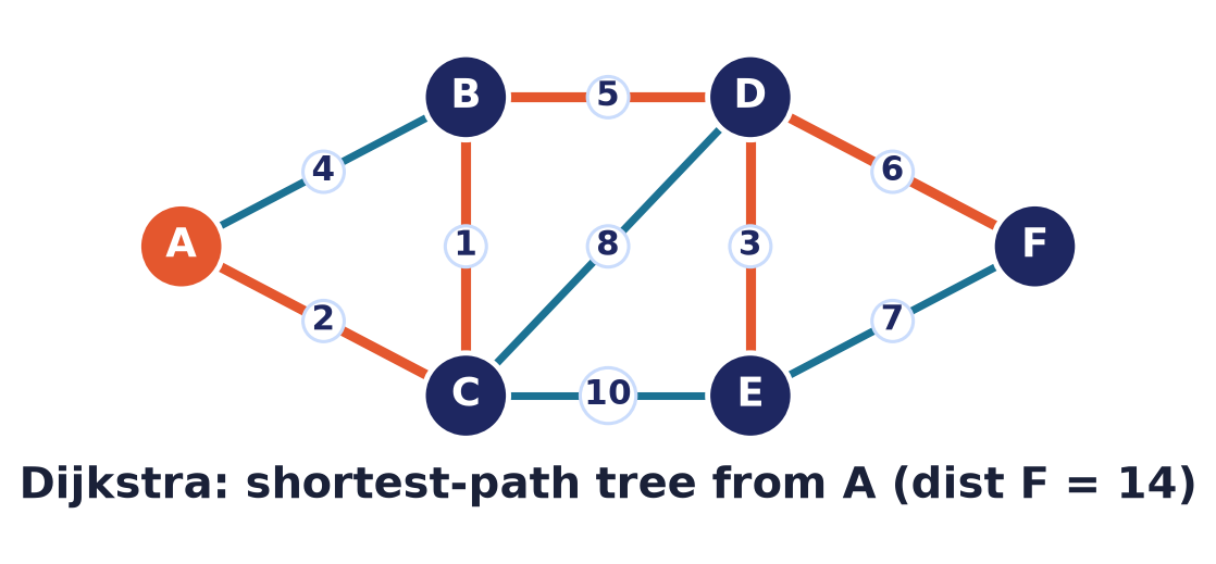
Final distances from : . Three separate vertices (, , ) had their distances improved after first being reached — the essence of relaxation — and ’s tempting-but-worse route through was discarded.
Path reconstruction. Follow backward from the target. For : , giving the shortest path of length . The pointers of all vertices together form the shortest-path tree rooted at .
Correctness
Two elementary facts first, then the main theorem.
Lemma A (upper-bound property). At all times , and once is finite it is the length of some actual – path. Proof. Initially and all others are . Relaxation only ever sets , which is the length of the path to (a real path, inductively) extended by edge ; and no real path can be shorter than the minimum .
Lemma B (subpath optimality). If is a shortest path, then each prefix is a shortest path to , so . Proof. A cheaper route to a prefix endpoint could be spliced in to beat the whole path, contradicting its optimality.
Theorem 11.5 (Dijkstra correctness). When Dijkstra extracts a vertex from , its distance is correct: . Hence all final distances are correct.
Proof (by contradiction on the extraction order). Suppose not, and let be the first vertex extracted with . By Lemma A, , so in fact . Note (since and is extracted first, correctly), and (otherwise ), so a shortest path from to exists.
Let be the set of vertices already finalized (extracted) just before is extracted. Then but , so starts inside and ends outside it. Walk along and let be the first vertex on that is not in , and let be its predecessor on (so ; possibly ).
Claim: . Since , was extracted before , and by our choice of as the first bad vertex, held at ’s extraction. At that moment we relaxed edge , so afterward . By Lemma B (as are consecutive on the shortest path ), . Thus , and with Lemma A, , proving the claim.
Now lies on at or before , and the piece of from to has non-negative total weight (this is the only place non-negativity is used!), so . Chaining the (in)equalities,
But both and are in when the algorithm chose to extract by minimum tentative distance, forcing — contradicting . No such exists, so every extraction is correct.
Why non-negativity is essential. The single step assumes the portion of costs . A negative edge breaks this, and Dijkstra can finalize a vertex too early.
Common pitfall — negative weights. Consider the directed graph (), (), (). Dijkstra extracts , sets , then extracts and finalizes at (it is the smallest), before ever examining . But the true shortest route is with length . Dijkstra never revisits a finalized vertex, so it reports — wrong. (If had any outgoing edge, the premature value would propagate, corrupting descendants too.) For graphs with negative edge weights use the Bellman–Ford algorithm, which relaxes every edge times in and, on a -th pass that still improves something, detects a negative-weight cycle (on which no shortest path exists).
Complexity
The running time depends entirely on the priority queue. Let and be the costs of extract-min and decrease-key. There are extractions and at most decrease-keys (one per relaxation), giving .
| Priority queue | extract-min | decrease-key | Total | Best for |
|---|---|---|---|---|
| Binary (min-)heap | general/sparse | |||
| Unsorted array | dense () | |||
| Fibonacci heap | * | * | theory / very large sparse |
(*amortized.) The workhorse is the binary heap, an array-embedded complete binary tree
in which every node’s key is its children’s; insert, decrease-key, and
extract-min each cost by sifting an element up or down one tree level at a
time. For a connected graph , so .
Remark (lazy deletion). Many implementations skip decrease-key: on each relaxation
they simply push a new pair and, on extraction, discard any pair whose
key exceeds the current . The heap may hold up to entries, but since
, the bound is still . This trades a little memory
for much simpler code and is what most standard libraries do.
Common pitfall. Do not “update in place then forget to re-heapify.” Either call a real
decrease-key, or use lazy deletion and check for stale entries at extraction — otherwise
the queue’s min is wrong.
CS connection. Dijkstra is the basis of link-state routing (OSPF, IS-IS) and of the “uniform-cost search” in AI; adding a goal-directed heuristic turns it into the A* search algorithm used in games and mapping.
11.8 Minimum spanning trees and the cut property
The problem
Anticipating Lecture 12: a spanning tree of a connected graph is a subgraph that is a tree (connected, acyclic) and includes every vertex; it necessarily has exactly edges. A minimum spanning tree (MST) is a spanning tree of least total edge weight. MSTs answer “what is the cheapest set of links that keeps the whole network connected?” — laying cable, roads, or pipelines; they also seed clustering algorithms and give a -approximation for the metric traveling-salesman problem.
Both algorithms that follow are greedy, and both are proved correct by a single lemma. To state it we need the vocabulary of cuts.
Cut. A cut is a partition of the vertices into two nonempty parts. Crossing edge. An edge crosses the cut if it has one endpoint in and the other in . Light edge. A crossing edge of minimum weight is a light edge of the cut. Respecting a cut. A set of edges respects the cut if no edge of crosses it. Safe edge. An edge is safe for if (some MST) implies (some MST).
The cut property
Theorem 11.6 (Cut Property). Let be a set of edges contained in some MST of . Let be any cut that respects, and let be a light edge crossing this cut. Then is safe for .
Proof (exchange argument). Let be an MST with . If we are done, since then . So suppose , with and .
Adding to the tree creates exactly one cycle (a fundamental fact about trees, Lecture 12: any two vertices already have a unique path in , and closes it into a cycle). Traversing , we start at , use to reach , and eventually return to ; since each crossing switches sides and we must end where we began, crosses the cut an even number of times. It crosses once at , so it crosses at least once more, at some edge .
This is not in : it crosses the cut, but respects the cut (no -edge crosses). Now exchange: set . Removing , an edge on the cycle , keeps connected; it still has edges, so is a spanning tree. Its weight is
Because is a light (minimum-weight) crossing edge and also crosses, , so . But is an MST, so ; hence and is also an MST. Finally (we removed and added ) and , so : the edge is safe.
Theorem 11.7 (Cycle Property). For any cycle in , if is a strict-maximum-weight edge of , then belongs to no MST. Proof. If some MST contained , deleting splits into two components; the rest of the cycle is a path joining ’s endpoints, so it contains some edge crossing that split with . Then is a spanning tree of smaller weight — contradiction.
The cut property tells us which edges to include; the cycle property tells us which to exclude. Prim and Kruskal are the two ways to apply the first; Kruskal also uses the second to justify skipping edges.
Corollary 11.8 (uniqueness). If all edge weights are distinct, the MST is unique. Proof. In Theorem 11.6 with distinct weights, a light edge would give strictly, hence , contradicting that is an MST — so every MST contains every light edge of every cut, pinning down one tree.
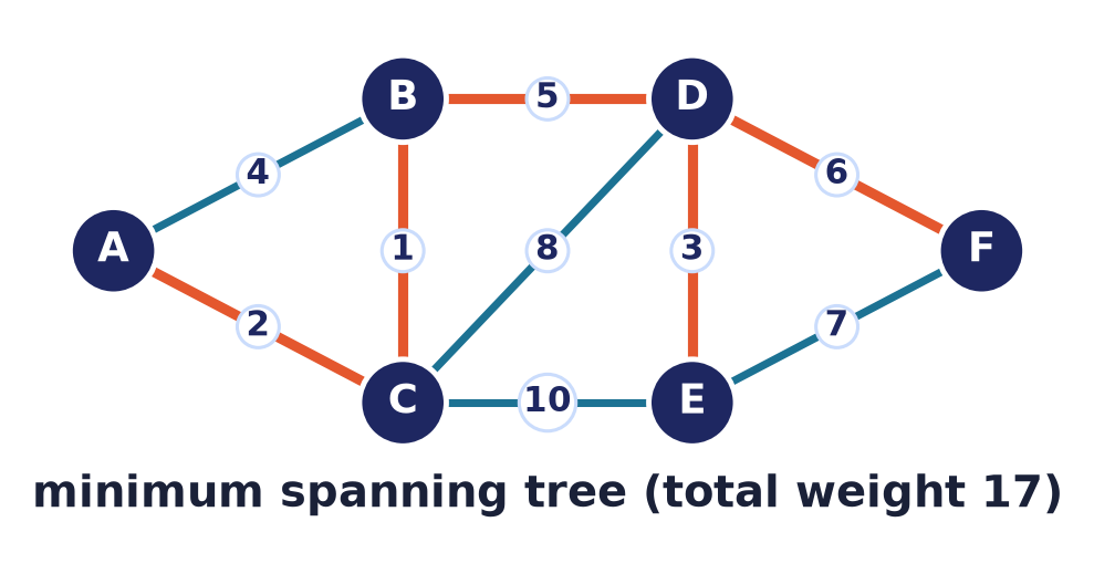
Because our running graph has distinct weights, its MST is unique, and Prim and Kruskal must produce identical edge sets, not merely equal weights.
11.9 Prim’s algorithm
Idea and pseudocode
Prim’s algorithm grows a single tree outward from a start vertex. It keeps the set of tree vertices and, at every step, adds the cheapest edge crossing from the tree to a vertex not yet in it. Each vertex outside the tree stores , the weight of the cheapest known edge connecting it to the current tree, and a priority queue delivers the global minimum.
function Prim(G, w, s):
    for each vertex v:
        key[v] ← ∞          # cheapest known edge connecting v to the tree
        parent[v] ← undefined
        inMST[v] ← false
    key[s] ← 0
    Q ← min-priority queue of all vertices, keyed by key
    while Q is not empty:
        u ← extract-min(Q)
        inMST[u] ← true
        for each neighbor v of u:
            if not inMST[v] and w(u, v) < key[v]:
                key[v] ← w(u, v)
                parent[v] ← u
                decrease-key(Q, v, key[v])
    return { (v, parent[v]) : v ≠ s }      # the MST edges
Worked trace
Run Prim on from . Each row shows the array after one extraction; “” marks a vertex now in the tree, and bold marks a key just improved. The Added edge is for the extracted .
| Step | Extracted | Added edge | ||||||
|---|---|---|---|---|---|---|---|---|
| 0 | — | — | ||||||
| 1 | — | 4 | 2 | |||||
| 2 | 1 | 8 | 10 | |||||
| 3 | 5 | |||||||
| 4 | 3 | 6 | ||||||
| 5 | ||||||||
| 6 |
Narration:
- Step 1 — from , keys of become .
- Step 2 — extract (key , cheapest), add . Relaxing ’s edges drops from to (edge ), and sets .
- Step 3 — extract (key ), add . Edge drops from to .
- Step 4 — extract (key ), add . Edge drops from to , and .
- Step 5 — extract (key ), add . Edge has weight , so is unchanged.
- Step 6 — extract (key ), add . Tree complete.
MST edges: ; total weight . Five edges for six vertices — a valid spanning tree. Notice Prim added the weights in the order : it takes the cheapest frontier edge, which is generally not the globally cheapest remaining edge (contrast Kruskal).
Correctness
Theorem 11.9. Prim’s algorithm returns a minimum spanning tree.
Proof. Let be the set of edges chosen so far, and the set of vertices in the tree (those with ). We prove the invariant is contained in some MST by induction on the steps.
Base. Initially for any MST .
Step. Assume some MST. Consider the cut . Every edge of joins two vertices that entered the tree, hence lies inside , so respects this cut. The next edge Prim adds is, by construction, the minimum-weight edge from to — a light edge of the cut. By the Cut Property (Theorem 11.6) this edge is safe, so is contained in some MST. The invariant is maintained.
When empties, and has edges forming a spanning tree contained in an MST; a spanning tree contained in an MST is that MST.
(The algorithm never gets stuck while : because is connected there is always at least one edge crossing the cut, so some vertex has finite key.)
Complexity
Structurally Prim is Dijkstra with a different key (“cheapest edge into the tree” instead of “distance from source”), so it has the identical cost profile:
- Binary heap: .
- Unsorted array: — preferred for dense graphs, since it is independent of .
- Fibonacci heap: .
Common pitfall. Prim needs the graph to be connected; on a disconnected graph it only spans the start vertex’s component (a minimum spanning forest requires restarting from each component). Also, only relax to vertices not yet in the tree — relaxing to in-tree vertices is wasted work and can corrupt keys if written carelessly.
11.10 Kruskal’s algorithm
Idea and pseudocode
Kruskal’s algorithm attacks the MST from the edges. It sorts all edges by increasing weight and scans them, adding an edge to a growing forest whenever it does not create a cycle — i.e. whenever its endpoints lie in different components. It stops after edges have been added.
The one nontrivial operation is testing “same component?” quickly, and updating components after a merge. That is exactly the job of a disjoint-set (union–find) data structure.
function Kruskal(G, w):
    A ← ∅                              # MST edge set
    for each vertex v: MakeSet(v)
    sort all edges of G by weight, ascending
    for each edge (u, v) in sorted order:
        if Find(u) ≠ Find(v):          # endpoints in different components
            A ← A ∪ { (u, v) }
            Union(u, v)
            if |A| = n - 1: break       # tree complete
    return A
The union–find (disjoint-set) data structure
Union–find maintains a partition of the vertices into disjoint sets — the components of the forest built so far — supporting three operations:
MakeSet(x)— put in its own singleton set;Find(x)— return a canonical representative (root) of ’s set; two elements are in the same set iff their representatives are equal;Union(x, y)— merge the two sets containing and .
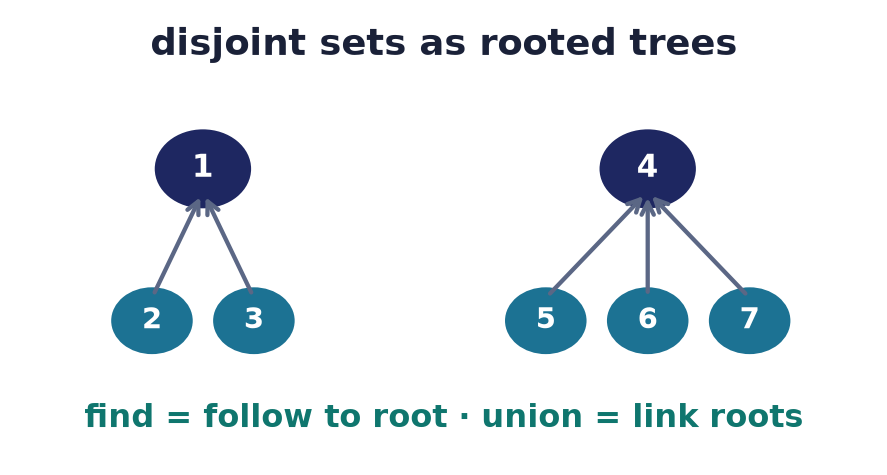
Each set is stored as a rooted tree via a parent array (the root points to itself); Find
walks parent pointers to the root. Two optimizations keep the trees flat:
- Union by rank — each root carries a
rank(an upper bound on its tree’s height).Unionhangs the lower-rank root under the higher-rank root, so the height grows only when two equal-rank trees merge. - Path compression — during
Find, re-point every node on the path directly to the root, so future queries are .
function Find(x):
    if parent[x] ≠ x:
        parent[x] ← Find(parent[x])    # path compression
    return parent[x]

function Union(x, y):
    rx ← Find(x);  ry ← Find(y)
    if rx = ry: return
    if rank[rx] < rank[ry]: swap(rx, ry)   # union by rank: attach smaller under larger
    parent[ry] ← rx
    if rank[rx] = rank[ry]: rank[rx] ← rank[rx] + 1
Complexity. With both optimizations, any sequence of operations on elements runs in time (Tarjan, 1975), where is the inverse Ackermann function — it grows so slowly that for every that could be written down in the physical universe. So each operation is effectively constant time, “near-linear” overall. (Either optimization alone gives per operation; together they are strictly better.)
A concrete union–find trace. Watch the structure through Kruskal’s unions on (shown next). Start with every vertex its own root, all ranks .
| Operation | Effect (parent / rank changes) | Roots afterward |
|---|---|---|
Union(B,C) |
equal ranks: , | |
Union(A,C) |
(rank 1) (rank 0): | |
Union(D,E) |
equal ranks: , | |
Union(B,D) |
equal ranks : , | |
Union(D,F) |
(rank 2) (rank 0): |
After these, a call to Find(E) walks and, by path compression, re-points
so the next Find(E) is a single hop — this is path
compression in action.
Worked trace
Same graph . Sorted edges: .
| Edge | vs | Cycle? | Action | Components after | |
|---|---|---|---|---|---|
| 1 | no | add | |||
| 2 | no | add | |||
| 3 | no | add | |||
| 4 | yes | skip | |||
| 5 | no | add | |||
| 6 | no | add | |||
| 7 | — | — | ( reached) | — | |
| 8 | — | — | — | — | |
| 10 | — | — | — | — |
MST edges: ; total weight .
This is exactly the tree Prim found (both equal , weight ) — as Corollary 11.8 guarantees, since ’s weights are distinct. The edge was skipped because and were already in the same component : adding it would close the cycle , on which is the heaviest edge.
Correctness
Theorem 11.10. Kruskal’s algorithm returns a minimum spanning tree.
Proof. Again we show the invariant the chosen set is contained in some MST, by induction on additions. The base case is immediate.
Suppose some MST and Kruskal is about to add edge because . Let be the component of in the current forest , and take the cut . Every edge of lies within a single component, so no -edge crosses this cut: respects it. Moreover crosses it (its endpoints are in different components, one being ).
Claim: is a light edge of this cut. Suppose some crossing edge had . Kruskal processes edges in increasing weight, so was examined earlier. Since crosses , its endpoints lie in different components now; and because components only ever merge (union–find never splits), they were in different components then too — so would have been added, i.e. . But then is an -edge crossing the cut, contradicting that respects it. Hence no crossing edge is lighter than ; is light.
By the Cut Property (Theorem 11.6), is safe: lies in some MST. The invariant holds. Skipped edges are harmless: an edge is skipped only when its endpoints are already connected by lighter edges, so it is the heaviest edge on the cycle it would close, and by the Cycle Property (Theorem 11.7) belongs to no MST. Finally, because is connected, Kruskal keeps finding cross-component edges until the forest becomes a single spanning tree of edges — an MST.
Complexity
- Sorting the edges dominates: (as gives ).
- Union–find:
MakeSet, and at mostFindplusUnion, all together — essentially linear, and dominated by the sort.
So Kruskal runs in . If the edges are already sorted, or weights are small integers sortable in by radix sort, the bottleneck disappears and Kruskal runs in — nearly linear.
Common pitfall. Omitting union by rank (or path compression) is a real trap: naive
Find up an unbalanced tree degrades to per query, making the union–find scan
and silently dominating the sort. Keep both optimizations.
Prim vs Kruskal
Both produce an MST; here both return of weight . They differ in the shape of the greed and in their ideal inputs:
- Prim grows one connected tree from a seed, always taking the cheapest edge on its frontier; it is vertex-driven via a priority queue. Its array version is , independent of , so it shines on dense graphs.
- Kruskal considers edges globally cheapest-first, gluing separate forest fragments; it is edge-driven via a sort plus union–find. It shines on sparse graphs and when edges arrive already sorted.
11.11 Comparison of all five algorithms
| Algorithm | Problem solved | Greedy step | Data structure | Time | Optimal? |
|---|---|---|---|---|---|
| Greedy vertex coloring | proper vertex coloring | smallest free color, per vertex | adjacency list + scratch array | no — colors | |
| Greedy edge coloring | proper edge coloring | smallest free color, per edge | adjacency list + scratch array | no — colors | |
| Dijkstra | single-source shortest paths, | finalize nearest, relax edges | binary heap (min-PQ) | yes | |
| Prim | minimum spanning tree | add cheapest frontier edge | binary heap (min-PQ) | yes | |
| Kruskal | minimum spanning tree | add cheapest cycle-free edge | sort + union–find | yes |
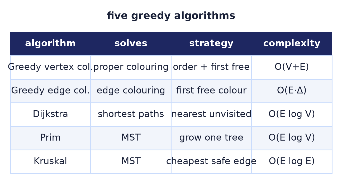
Threads running through the table:
- Greedy is universal here, but its guarantees differ. For shortest paths and MSTs a greedy step is provably safe — via the finalized-distance invariant (Theorem 11.5) and the cut property (Theorem 11.6). For coloring, greedy is only a bounded, order-sensitive approximation (Theorems 2, 4).
- Dijkstra and Prim are structural twins. Both loop “extract the cheapest vertex, then relax its edges,” differing only in the meaning of the key: distance from the source (Dijkstra) versus weight of the cheapest edge into the tree (Prim). Their complexity profiles are identical. Kruskal is different in kind — edge-driven, needing union–find.
- Watch the assumptions. Dijkstra requires non-negative weights (else Bellman–Ford); Prim and Kruskal require a connected graph (else they build a spanning forest); distinct weights make the MST unique.
Historical notes
- Otakar Borůvka (1926) posed and solved the MST problem first, to lay an efficient electrical grid in Moravia; his parallel-flavored algorithm predates the others by decades.
- Vojtěch Jarník (1930) described the tree-growing method now usually credited to Prim.
- Joseph Kruskal (1956) published “On the shortest spanning subtree of a graph and the traveling salesman problem.”
- Robert C. Prim (1957), at Bell Labs, rediscovered Jarník’s method; Edsger W. Dijkstra (1959) rediscovered it again and published his shortest-path algorithm in the same three-page note (Numerische Mathematik 1). Dijkstra later recalled designing the shortest-path algorithm in about twenty minutes, in his head, at an Amsterdam café. Because of this triple origin, Prim’s algorithm is sometimes called the Jarník–Prim or DJP algorithm.
- R. L. Brooks (1941) proved except for complete graphs and odd cycles; Vadim G. Vizing (1964) proved ; Welsh and Powell (1967) introduced the largest-degree-first coloring heuristic in a paper on timetabling.
- The union–find structure was introduced by Galler and Fisher (1964); its near-linear analysis is due to Hopcroft and Ullman (1973) () and, tightly, to Robert Tarjan (1975) (), with a matching lower bound by Fredman and Saks (1989).
Chapter summary
- Every optimization algorithm here is greedy (the BFS/DFS traversals aside). For shortest paths and MSTs, greed is provably optimal; for coloring, it is only a bounded, order-dependent heuristic.
- Breadth-first and depth-first search are the two systematic traversals: BFS explores in rings of increasing distance (a queue — and shortest paths in unweighted graphs), DFS plunges as deep as possible before backtracking (a stack/recursion). Both run in and underpin connectivity, component counting, and the tree/shortest-path algorithms below.
- Greedy vertex coloring processes vertices in some order, assigning each the smallest color free among colored neighbors. It is always proper (Theorem 11.1), uses colors (Theorem 11.2, hence ), runs in , but its color count depends on the order — on , one order used (optimal), another . Welsh–Powell (largest degree first) is a good default.
- Greedy edge coloring is the same idea on the line graph: always proper, colors, . Vizing bounds the true optimum by ; on , greedy achieved , its classes forming matchings (one perfect).
- Dijkstra solves single-source shortest paths for non-negative weights by repeatedly finalizing the nearest vertex and relaxing its edges. Theorem 11.5 proves each finalized distance is correct via a shortest-path invariant, using non-negativity at exactly one step. With a binary heap it runs in . Negative weights break it — use Bellman–Ford (, detects negative cycles). On from : .
- MSTs are governed by the Cut Property (Theorem 11.6): a light edge across any cut respected by the current edge set is safe. This one lemma proves both Prim (grow one tree, add the cheapest frontier edge) and Kruskal (add globally cheapest cycle-free edges) correct. The Cycle Property justifies Kruskal’s skips. On both give the same unique MST of weight .
- Union–find with union by rank + path compression supports Kruskal’s cycle tests in amortized — effectively constant. Kruskal’s cost is dominated by the edge sort. Prim and Kruskal are the two greedy faces of the same optimization.
Exercises
Use the running graph (vertices –; edges and weights in the table above) unless a problem says otherwise.
Warm-up
- Starting from vertex and visiting neighbours in alphabetical order, give the vertex-discovery order for (a) breadth-first and (b) depth-first search on . How many edges does each search tree contain, and why?
- Run greedy vertex coloring on in the order . How many colors does it use? Compare with the natural order .
- State the two greedy upper bounds — colors for vertices, for edges — and explain in one sentence each where the bound comes from.
- Run Dijkstra on from source . Give the final distance to every vertex and the shortest path to .
- What are and ? For each, give the lower-bound argument that proves the value greedy found is optimal.
- In Kruskal’s trace on the edge was skipped. Which
Findcomparison caused the skip, and which cycle would have closed? - List the MST edges and total weight produced by (a) Prim from and (b) Kruskal. Are the edge sets identical, and why is that guaranteed here?
Standard
- Apply Welsh–Powell to (break degree ties alphabetically) and give the resulting coloring. Does it match the optimum?
- Prove that greedy vertex coloring always yields a proper coloring, for every ordering.
- Prove the bound and state the graph ’s values of and to show the bound need not be tight.
- In the Dijkstra trace, vertex was finalized at , though it was first reached with tentative value . Identify the relaxation that improved it, and explain why the later edge did not change .
- Give a small directed graph with one negative edge on which Dijkstra returns a wrong distance; show Dijkstra’s output and the true distance, and name the algorithm you would use instead.
- State the Cut Property and use it to justify Prim’s first edge choice on (from ): exhibit the cut and the light edge.
- Perform Kruskal’s
Unionoperations on using union by rank + path compression. Give the finalparentandrankarrays, and describe whatFind(E)returns and how it compresses the path. - Suppose the weight of is lowered from to . Recompute the MST (edges and weight) and say which edge leaves the tree and why.
Challenge
- Prove the Cut Property (Theorem 11.6) in full, including the claim that a cycle crosses any cut an even number of times.
- Prove Dijkstra’s correctness (Theorem 11.5) and pinpoint the single step that requires non-negative edge weights.
- Prove that if all edge weights are distinct, the MST is unique. (Hint: combine the cut and cycle properties, or run an exchange argument.)
- For the crown graph ( minus a perfect matching), prove that the ordering forces greedy to use colors, although . What does this say about the tightness of the bound?
- Prove that union by rank alone (no path compression) keeps every tree of height with
at least nodes, hence
Findcosts . - Sketch the Bellman–Ford algorithm: its relaxation loop, why passes suffice on graphs without a negative cycle, how a -th improving pass detects a negative cycle, and its running time. Why is Dijkstra preferred when weights are non-negative?
Selected answers & hints
1. Both searches start at . (a) BFS discovers vertices in nondecreasing distance from the source (a queue); (b) DFS dives as deep as possible before backtracking (a stack/recursion). Each search tree has edges — a spanning tree of the connected graph — since every non-root vertex is reached across exactly one tree edge; the exact discovery order depends on the adjacency list.
2. Order gives — 3 colors, same count as the natural order (both optimal, since ). The specific color labels differ, but the number does not.
3. Vertex: a vertex has colored neighbors, so one of colors is always free. Edge: an edge is adjacent to other edges, so one of is always free.
4. From the extraction order is ; final distances . Shortest path to : (weight ).
5. : the triangle forces , and greedy exhibits a proper -coloring. : vertex has degree , so its four incident edges need distinct colors (), and greedy exhibits a proper -edge-coloring.
6. When is examined, (both are in the component formed by adding then ), so it is skipped; it would close the cycle , on which it is the heaviest edge ().
7. Both give , weight . The sets are identical because all nine weights are distinct, so the MST is unique (Corollary 11.8).
11. was first set to when was finalized (edge , ); it improved to when was finalized and edge gave . Later, from , edge offers , which is (set via ), so no update.
12. Directed . Dijkstra finalizes at (it is the current minimum) before examining , so it reports ; but costs , the true distance. Use Bellman–Ford for negative weights.
14. Processing unions yields root
with ; : .
Find(E) walks , returns , and by path compression sets
(so a subsequent Find(E) is one hop).
15. Lowering to makes it the cheapest edge; the new MST is of weight . The edge leaves: in Kruskal, now precedes it and already connects ; equivalently, on the cycle the heaviest edge is now , which the cycle property excludes.
18. If two distinct MSTs existed, take the minimum-weight edge in their symmetric difference, say . Adding to makes a cycle; by distinctness some cycle edge has (else would not be minimal in the difference), and swapping for gives a lighter spanning tree than — contradiction. Hence the MST is unique.
19. By induction: gets ; (non-adjacent to ) gets ; and when we reach their already-colored neighbors are exactly minus the one partner they miss, which carry all of colors — so both get . Thus greedy uses colors while , showing the (here ) bound and the general optimality gap can be enormous under an adversarial order.
21. Bellman–Ford relaxes all edges, repeated times; since any shortest path has at most edges and each full pass correctly settles one more edge along it, passes suffice when there is no negative cycle. If an -th pass still relaxes some edge, a negative-weight cycle is reachable (distances would otherwise be stable), so report it. The cost is . Dijkstra’s is far better, so prefer it whenever all weights are .
Further reading
- Rosen, Discrete Mathematics and Its Applications — §11.6 (shortest-path problems and Dijkstra’s algorithm), §11.8 (graph coloring), and §11.4–11.5 (spanning trees and minimum spanning trees, with Prim’s and Kruskal’s algorithms). Matches this course’s level and notation.
- Cormen, Leiserson, Rivest, and Stein (CLRS), Introduction to Algorithms — the chapters on Minimum Spanning Trees (Kruskal and Prim), Single-Source Shortest Paths (Bellman–Ford and Dijkstra), and Data Structures for Disjoint Sets (union–find with the analysis). In the 3rd edition these are Chapters 23, 24, and 21 respectively. The definitive source for the correctness proofs and complexity bounds sketched here.