Lecture 13. Probabilities
13.1 Overview
Every branch of mathematics we have met so far describes a deterministic world: a set either contains an element or it does not (Lectures 1–2), two elements are either related or they are not (Lecture 3), a proposition is either true or false (Lecture 6). Probability theory is the branch of discrete mathematics that extends this black-and-white logic to a world of graded certainty — it attaches to each uncertain statement a number between and measuring how likely it is to be true.
Why should a computer scientist care? Because the most powerful ideas in modern computing are probabilistic:
- Randomized algorithms (quicksort with a random pivot, randomized primality testing, skip lists, hashing) trade a tiny chance of a bad outcome for dramatic speed. Analysing them means computing and showing it is negligible.
- Hashing and load balancing live or die by collision probabilities — the birthday problem of this lecture is exactly the analysis of a hash table.
- Machine learning is applied probability: a spam filter computes with Bayes’ theorem; a classifier’s precision and recall are conditional probabilities.
- Cryptography rests on the infeasibility of guessing a random key, and the “birthday attack” is a direct application of the birthday problem.
- Networks, queues, and reliability are modelled by the probability that a packet is lost, a server is busy, or a component fails.
This lecture builds finite (discrete) probability from the ground up in three stages.
- Language. Random experiments, the sample space , and events — which turn out to be nothing more than the sets of Lecture 1, so the whole algebra of Lecture 2 transfers verbatim.
- Measure. How to attach a number to an event: the classical (Laplace) ratio, the counting tools (combinatorics) needed to evaluate it, and the three axioms of Kolmogorov that pin down what “probability” is.
- A calculus of events. Theorems that combine probabilities — the complement rule, the addition rule (a probabilistic inclusion–exclusion), conditional probability, the multiplication rule, independence, the law of total probability, and Bayes’ theorem — each stated precisely and proved from the axioms.
We close with three celebrated problems every student should meet once — the birthday problem, the Monty Hall problem, and a Bayesian medical-test calculation — and a first look at random variables and expectation.
Throughout we stay in the discrete, finite world: the sample space has finitely many outcomes. Continuous distributions (the normal curve, densities, integrals) are the subject of a later course and are out of scope here.
13.2 Random experiments, sample space, and events
A random experiment (trial) is a process whose individual outcome cannot be predicted with certainty in advance, even though the set of possible outcomes is known and the experiment can (in principle) be repeated under identical conditions. Tossing a coin, rolling a die, drawing a card, and picking a ball from an urn are the classic examples; so is “hash a random key into a table of size ” or “run randomized quicksort on this array.”
The sample space (also written or ) is the set of all possible outcomes of the experiment. Each individual outcome is an elementary event (sample point) — an outcome that cannot be decomposed further.
An event is any statement about the experiment that becomes definitely true or false once the outcome is known — formally, a subset . The event occurs exactly when the realized outcome belongs to . An event containing more than one elementary outcome is a compound event.
Example (die). Roll one fair six-sided die, so and . The elementary event “roll a ” is the singleton . The compound event “even number” is ; “greater than ” is . Then , , and .
Example (two coins). Toss two distinguishable coins: , . The event “exactly one head” is . Note that this is the Cartesian product from Lecture 2 — building compound sample spaces out of simple ones is exactly the product construction.
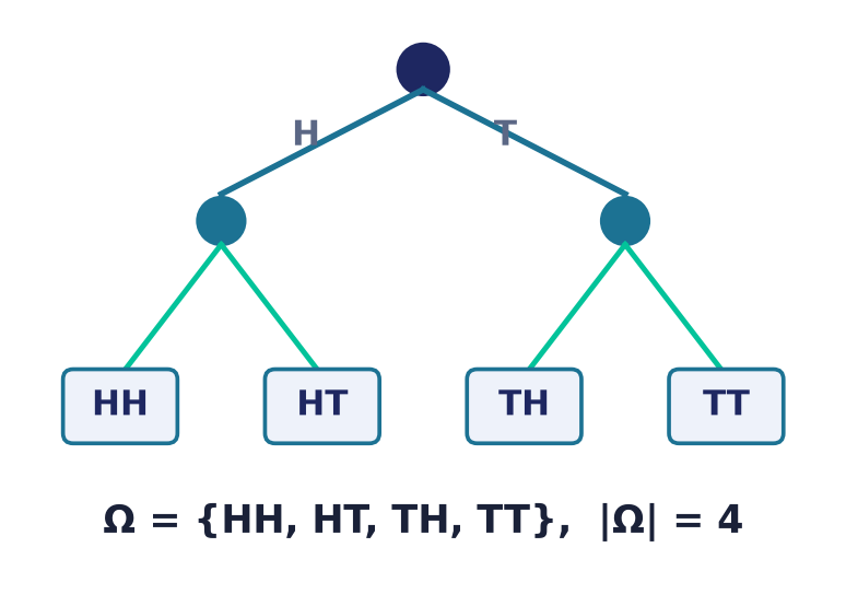
Events are sets: the algebra of events
Because an event is a subset of , the set operations of Lectures 1–2 carry over with no change — only the reading changes. This dictionary is the single most useful table in the lecture; keep it in view.
| Set notation | Event language | “occurs when…” |
|---|---|---|
| outcome makes occur | the realized outcome lies in | |
| certain event | always | |
| impossible event | never | |
| “ or ” (at least one) | or | |
| (also ) | “ and ” (both) | and |
| “not ” | ||
| “ implies ” | whenever occurs, so does | |
| mutually exclusive | they cannot co-occur | |
| “ but not ” | and |
Consequently De Morgan’s laws from Lecture 2 read, in event language,
Remark (why “events as sets” matters). This is not a coincidence to be admired and forgotten. Every probability manipulation below is first a set manipulation and then an application of an axiom. When a word problem confuses you, translate it into set operations on first; the arithmetic follows.
Remark (the event space). For a finite we take every subset to be an event, so the collection of events is the power set (Lecture 1), with events in all. For infinite sample spaces one cannot always take every subset and must restrict to a so-called -algebra; that subtlety never arises in the finite world of this lecture.
13.3 Types of events
Classifying how events relate to one another decides which rule applies later, so the vocabulary is worth stating precisely.
Certain (reliable) event — occurs in every trial. It is the whole sample space and (we will prove) has probability . Example: “the die shows a number in .”
Impossible event — never occurs. It is the empty set and has probability . Example: “the die shows .”
Compatible (jointly possible) events — can occur in the same trial: . On one die, “even” and “greater than ” share the outcome , so they are compatible.
Incompatible (mutually exclusive) events — cannot occur together: (the disjoint sets of Lecture 2). “Roll a ” and “roll a ” cannot both happen in one roll. Distinct elementary events are always pairwise incompatible.
A family of events forms a complete group (a partition of ) if they are pairwise incompatible and their union is — so exactly one of them occurs in every trial. This is precisely the partition concept of Lecture 3, where a partition of a set arose as the family of equivalence classes of an equivalence relation. There, blocks were “elements that are equivalent”; here, blocks are “outcomes that trigger the same hypothesis.” The idea returns as the backbone of the total-probability formula.
Complementary (opposite) events — the special case of a complete group of two: and are incompatible and together exhaust . Example: “the die shows ” and “the die does not show .” We will prove .
Independent events — the occurrence of one does not change the probability of the other (made precise below). Drawing a ball, replacing it, then drawing again gives independent draws.
Dependent events — the occurrence of one does change the probability of the other. Drawing two balls without replacement makes the second draw depend on the first.
Common pitfall. Independence is not the same as incompatibility — in fact they are almost opposites. We will prove that two incompatible events of positive probability are necessarily dependent: if occurs then has become impossible, which is a maximal change in ’s probability. Do not equate “” with “ independent.”
13.4 The classical (Laplace) definition of probability
When a finite experiment has equally likely elementary outcomes, of which exactly are favourable to an event , the classical (Laplace) probability of is
The “equally likely” hypothesis is essential and is justified by symmetry: a fair coin, a fair die, a well-shuffled deck, and a thoroughly mixed urn have no physical reason to prefer one outcome over another. Where symmetry fails, the classical definition does not apply and we fall back on the statistical definition below.
Example (die). , since of the equally likely faces are even.
Example (cards). From a standard -card deck, and (the jacks, queens, kings).
Because , the ratio always lies in ; and . The whole of classical probability therefore reduces to a counting problem — “how many favourable, how many total?” — which is why we develop combinatorics next.
Statistical (frequentist) probability. When symmetry fails (a bent coin, an unknown manufacturing process) we estimate probability empirically. If in independent trials the event occurs times, its relative frequency is . The law of large numbers says that as this frequency stabilizes around a fixed number, the statistical probability . For fair mechanisms the statistical and classical values agree; the statistical view is what lets us speak of “the probability of rain” or “the probability a hard drive fails within a year,” where no symmetry is available.
13.5 Counting: combinatorics as the engine of classical probability
To use we must count outcomes. Three counting devices — resting on one master principle — handle almost every finite problem. Throughout, is the number of available objects and the number chosen.
The multiplication principle (rule of product)
Multiplication principle. If a procedure consists of successive steps, where step can be done in ways, step in ways regardless of the first choice, …, and step in ways regardless of the earlier choices, then the whole procedure can be carried out in
Proof. An outcome of the procedure is precisely a -tuple with one of the choices at step , so the set of outcomes is the Cartesian product of Lecture 2 with . The cardinality of a finite Cartesian product is the product of the cardinalities, , which one proves by induction on : the case is immediate, and because each of the shorter tuples extends in exactly ways. ∎
Example. A password of lowercase letters followed by digits can be formed in ways. Rolling two dice yields ordered outcomes — the sample space .
Permutations
Permutation of objects — an ordering (in a row) of all distinct objects. The number of permutations is
Proof. Filling the positions left to right is a -step procedure: the first position admits choices, the second (one object is used up), …, the last . By the multiplication principle the count is . ∎
-permutation (arrangement) — an ordered selection of out of distinct objects (order matters, no repetition). Its count, written (the notation used in Rosen; the same quantity appears in the European tradition as , the number of arrangements), is
Proof. Fill ordered positions from objects: choices for the first, for the second, …, for the -th. The product of these factors is , which equals after cancelling the tail . ∎
Example. Choosing a president and then a (distinct) secretary from people gives ordered pairs. All orderings of books on a shelf: .
Combinations
Combination — an unordered selection of out of distinct objects (order does not matter, no repetition), i.e. a -element subset. Its count is the binomial coefficient
Proof. Count ordered -selections two ways. On one hand there are of them. On the other hand, to build an ordered selection we may first choose the set of objects — say there are such sets — and then order them, which by the permutation count can be done in ways. By the multiplication principle , so
Example. A committee of from people: . (Contrast with the ordered count ; dividing by removes the ordering.)
Two facts we will reuse:
- Symmetry: , since choosing the objects to include is the same as choosing the objects to exclude.
- Pascal’s identity: .
Proof of Pascal’s identity (combinatorial). Fix one particular object among the . Every -subset either contains or not. Those containing are formed by choosing the remaining members from the other objects: of them. Those not containing choose all members from the other : of them. These two cases are disjoint and exhaustive, so their counts add. ∎
Common pitfall (a notation clash). The letter is overloaded: is the probability of an event , while is the number of -permutations. They are told apart only by what sits inside the parentheses (a set/event vs. two integers). To avoid confusion this lecture writes probabilities of named events, e.g. , and permutation counts with two integer arguments, e.g. . The European-tradition notation , sidesteps the clash entirely.
Order matters? The single question that selects the tool: does rearranging the chosen objects give a different outcome? Yes ⇒ permutation ; No ⇒ combination . “President and secretary” is ordered; “a committee” is not.
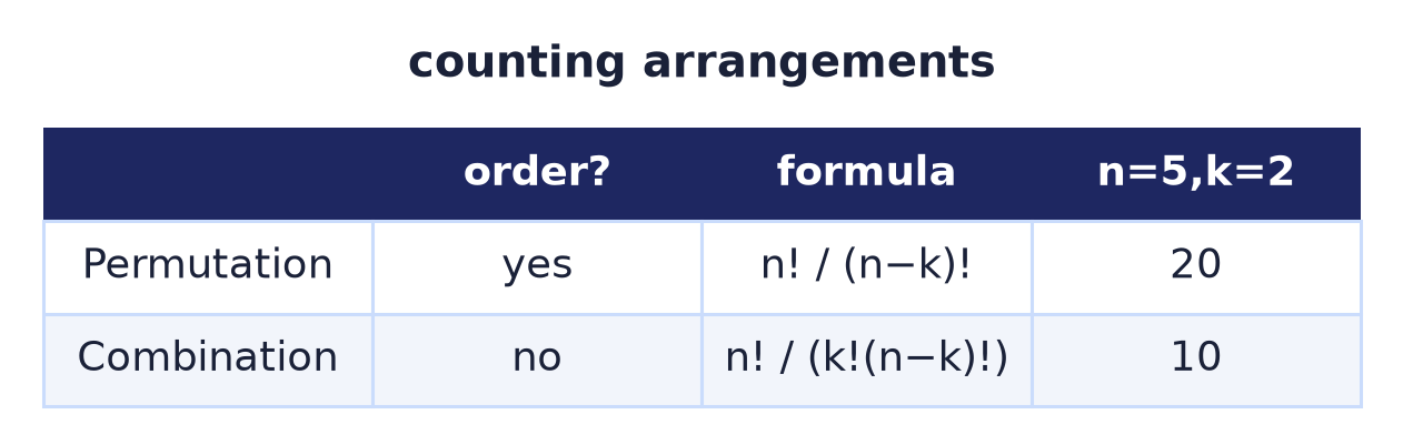
Example (urn, counting). An urn holds white and black balls; draw at once (order irrelevant). Total selections: . Favourable to “exactly white and black”: choose the whites ways and the black ways, giving . Hence
(This is a hypergeometric count — sampling without replacement — and we return to it below.)
Three more counting tools
- Sum rule (addition principle). If an object comes from one of disjoint cases with options, the total is . “Or / separate cases” adds, where the product rule’s “and / in stages” multiplies.
- Selections with repetition (multisets / stars-and-bars). Choosing objects from
types with repetition allowed — equivalently, distributing identical balls
into distinct boxes — is counted by
(line up stars and bars). This fills the last cell of the order-vs-repetition taxonomy: unordered with repetition.
- Binomial theorem. The combinations are the coefficients of a binomial power:
whence (put ) and the binomial-distribution weights sum to (put ).
13.6 Kolmogorov’s axioms
The classical ratio works only for equally likely outcomes and only for finite spaces. In 1933 A. N. Kolmogorov gave probability the abstract, symmetry-free foundation still used today: probability is any function on events obeying three axioms.
Definition (probability measure). A probability on a finite sample space is a function assigning to every event a real number such that
- (Non-negativity) for every event ;
- (Normalization) ;
- (Additivity) if then ; more generally, for pairwise incompatible events (finitely or countably many),
Everything else in this lecture is a theorem deduced from these three lines. Nothing about “equally likely” is assumed; the classical model is just one instance.
Building a finite probability space. On a finite it suffices to assign each outcome a weight with , and then define . Additivity then holds automatically. The classical (uniform) model is the special case for all .
Theorem (the classical ratio is a probability). For finite with , the function satisfies the three axioms.
Proof. Non-negativity: , so . Normalization: . Additivity: if then — this is exactly the disjoint-union counting rule of Lecture 2 — so . ∎
13.7 Derived rules and their proofs
We now prove, purely from Axioms 1–3, the working rules of probability. These proofs are the mathematical heart of the lecture; each is short, and together they show how much structure three axioms already force.
Theorem (finite additivity). If are pairwise incompatible then .
Proof. Induction on . The case is Axiom 3. Assume the claim for and let be pairwise incompatible. Put . Then , so by Axiom 3 and the induction hypothesis
Theorem (impossible event). .
Proof. and , so is incompatible with itself. Axiom 3 gives . Subtracting from both sides yields . ∎
Theorem (complement rule). For every event , .
Proof. and are incompatible () and exhaust the space (). By Axiom 3 and then Axiom 2,
so . ∎
This is the workhorse behind every “at least one” computation, because the complement “none” is usually far easier to count.
Theorem (range of probability). For every event , .
Proof. The lower bound is Axiom 1. For the upper bound, the complement rule gives , and by Axiom 1, so . ∎
Theorem (monotonicity and difference). If then and hence .
Proof. Since , the set splits as the disjoint union with . Axiom 3 gives , whence . As by Axiom 1, we get . ∎
Theorem (addition rule / inclusion–exclusion for two events). For any two events,
Proof. Write as the disjoint union , so by Axiom 3
Now , and splits as the disjoint union (an outcome of is either also in or not), so by Axiom 3
Substituting (2) into (1) gives . ∎
Remark. This is the probabilistic twin of the cardinality identity proved in Lecture 2; dividing that by in the classical model recovers it. The overlap is subtracted because outcomes in it are counted once in and again in . For incompatible events , the term vanishes and we recover .
Theorem (inclusion–exclusion for three events).
Proof. Apply the two-event rule to and :
Expand . For the last term, distributivity (Lecture 2) gives , so by the two-event rule again
and . Combining the pieces gives the stated formula. ∎
Theorem (Boole’s inequality / union bound). For any events ,
Proof. Induction on . For it is an equality. Assume it for . Writing , the two-event addition rule gives , since . By the induction hypothesis , so . ∎
CS connection. The union bound is the single most-used inequality in the analysis of randomized algorithms. If an algorithm fails only when at least one of “bad events” happens, and each has tiny probability , then the total failure probability is at most — no independence assumptions needed. Its power is that it needs nothing about how the interact.
13.8 Worked problems I: dice, cards, urns
We consolidate the rules so far on the three workhorse experiments, easy to hard. Every number is verified.
Problem 1 (single die, warm-up). Roll one fair die. Then and, since “roll or ” are incompatible, .
Problem 2 (two dice, the sum distribution). Roll two fair dice; equally likely ordered pairs. Counting the pairs with gives the full distribution:
| Sum | 2 | 3 | 4 | 5 | 6 | 7 | 8 | 9 | 10 | 11 | 12 |
|---|---|---|---|---|---|---|---|---|---|---|---|
| favourable pairs | 1 | 2 | 3 | 4 | 5 | 6 | 5 | 4 | 3 | 2 | 1 |
The counts sum to , confirming the probabilities total . The most likely sum is (six ways: ), giving .
Problem 3 (at least one six — complement). Roll two dice. (each die independently avoids six), so by the complement rule . Direct enumeration confirms of the pairs contain a six.
Problem 4 (cards, addition rule). Draw one card from .
subtracting the king of hearts, counted in both.
Problem 5 (cards, two aces). Draw cards without replacement. Counting unordered hands, . The sequential view agrees: .
Problem 6 (cards, at least one ace in a 5-card hand — complement).
Problem 7 (urn without replacement, hypergeometric). An urn has white and black balls; draw without replacement.
| Event | Count | Probability |
|---|---|---|
| all white | ||
| exactly white, black | ||
| exactly white, black | ||
| no white ( black) |
The four cases partition the outcomes: , so the probabilities sum to . ✓
Problem 8 (De Méré’s problem, historical, hard). The Chevalier de Méré, a 17th-century gambler, asked Pascal about two bets that “should” have equal odds:
- Bet A: at least one six in four rolls of one die.
- Bet B: at least one double-six in twenty-four rolls of two dice.
Using the complement rule and independence of rolls,
So Bet A is (barely) favourable and Bet B (barely) unfavourable — a difference of about percentage points that de Méré had detected empirically at the gaming table. The correspondence Pascal and Fermat exchanged to resolve such puzzles in 1654 is usually taken as the birth of probability theory.
13.9 Conditional probability
Often we learn partial information — a related event is known to have occurred — and must revise the probability of accordingly.
Definition (conditional probability). For events with , the conditional probability of given is
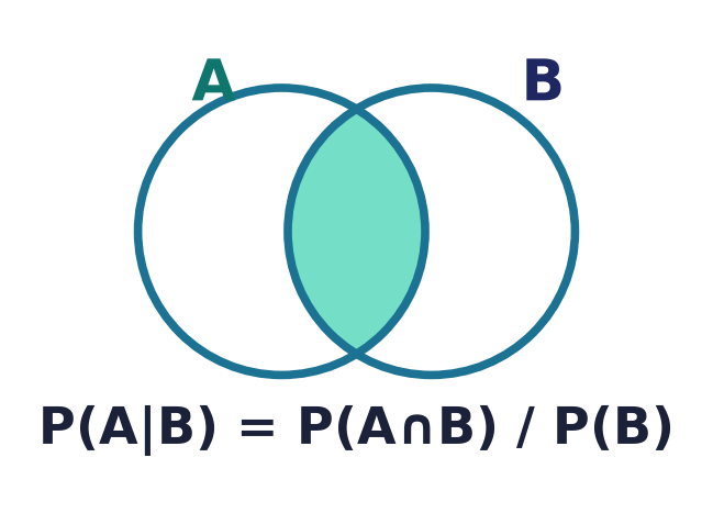
Intuition. Learning that occurred shrinks the world from down to : outcomes outside are now impossible. We rescale so that carries the full probability (divide by ) and ask what fraction of ’s probability also lies in (the numerator ). In the classical model this is transparent: — literally “favourable-within- over size-of-.”
Example (die). With “roll a ” and “even”: . Knowing the roll is even lifts the chance of a from to , because only three outcomes remain.
Remark (conditioning yields a probability). For fixed with , the map is itself a probability measure on : it is non-negative, assigns , and is additive over incompatible events. So every theorem proved above (complement rule, addition rule, …) holds inside a conditional world.
The multiplication rule and the chain rule
Rearranging the definition removes the fraction and gives the probability that both events occur.
Multiplication rule. For ,
This generalizes to any number of events.
Theorem (chain rule / general multiplication rule). For events with ,
Proof. Induction on . The case is the multiplication rule. Assume the identity for and write ; note implies each earlier intersection is positive too, by monotonicity. Then
and expanding by the induction hypothesis gives exactly the stated product. ∎
Example (draws without replacement, dependent). A box holds white and red balls ( total); draw without replacement. With “first white,” “second white,”
The draws are dependent: removing a white ball changes the second draw’s odds from to .
Example (defective parts, dependent). of parts are defective, so are non-defective; of the non-defective parts, are low quality. The probability a random part is non-defective and low quality is, by the multiplication rule, .
Example (two children — a conditional-probability pitfall). A family has two children; assume the four birth orders are equally likely.
- Given that at least one child is a boy, what is ? The condition is (three equally likely outcomes) and “both boys” is , so the answer is .
- Given that the elder child is a boy, what is ? Now the condition is and the answer is .
The two questions sound alike but condition on different events, and the answers genuinely differ. This is the classic warning that in the event must be pinned down exactly.
Common pitfall (transposing the conditional). and are different numbers; equating them is the prosecutor’s fallacy. “The probability of this DNA match if the suspect is innocent is in a million” () is not “the probability the suspect is innocent given the match” (). Bayes’ theorem below is exactly the machine for converting one into the other, and it shows they can differ by orders of magnitude when the base rates differ.
Common pitfall ( vs ). The conditional presumes has happened and lives in the shrunken world ; the joint makes no such assumption and lives in all of . They are related by a factor of and are equal only when .
13.10 Independence
Definition (independence of two events). Events and are independent if
Equivalently, when , this says : knowing tells us nothing new about .
Independence is often justified physically (separate coins, distinct dice, draws with replacement, independently chosen hash keys), but the defining equation is the formal test — and physical intuition can mislead, so when in doubt, check the equation.
Example (independent, product rule). Roll a die twice: , matching direct enumeration of the outcomes.
Example (two boxes, independent). Box 1 has white and red ( total); Box 2 has white and red ( total). Draw one ball from each. With “white from Box 1” and “white from Box 2” the draws are independent, so
Theorem (incompatible independent). If are incompatible and both have positive probability, then they are dependent.
Proof. Incompatibility means , so . But independence would require , since both factors are positive. The two are contradictory, so cannot be independent. ∎
This confirms the warning from the start of the lecture: incompatible events with positive probability are as far from independent as possible — the occurrence of one drives the other’s conditional probability to .
Remark (mutual vs. pairwise independence). For three or more events, pairwise independence (every pair satisfies the product rule) is weaker than mutual independence, which requires the product rule for every sub-collection, e.g. as well as the three pairwise equations. There are standard examples (two independent fair coins with “the coins agree”) that are pairwise but not mutually independent. Independence of “steps” in the multiplication principle is what makes valid, as in the “at least one six” and De Méré computations.
Example (lottery — dependent and compatible). Of tickets, win; you buy . Find . The two “this ticket wins” events are compatible and dependent (sampling without replacement). The complement route is cleanest:
The general addition rule agrees: with and , . ✓
13.11 The law of total probability
Suppose a first stage of an experiment produces one of several hypotheses (causes, scenarios), and a later event has known probability under each. The law of total probability assembles these into .
Theorem (law of total probability). Let form a complete group (partition of ): pairwise incompatible, , and each . Then for any event ,
Proof. Because the cover ,
using distributivity (Lecture 2). The sets are pairwise incompatible, since for . By finite additivity and then the multiplication rule (, valid as ),
Read it as a weighted average: the chance of is the average of its conditional chances , each weighted by how likely its hypothesis is.
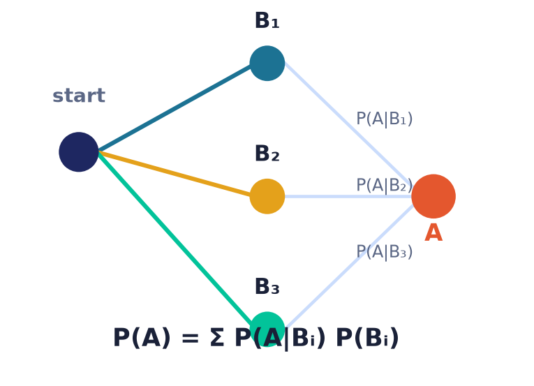
Example (choose an urn, then a ball). Urn 1 holds white and red; Urn 2 holds white and red. Pick an urn at random () and draw one ball. The probability it is white:
A probability tree organizes exactly this computation — first branch on the hypothesis, then on , multiply along a path, add across paths ending in :
                 P(W|H1)=2/12
        P(H1)=1/2 ─────────── White   path prob = 1/2 · 2/12 = 2/24
       ┌──────── Urn 1
       │         └─────────── Red     1/2 · 10/12 = 10/24
 start ┤
       │         ┌─────────── White   1/2 · 8/12  = 8/24
       └──────── Urn 2
        P(H2)=1/2 ─────────── Red     1/2 · 4/12  = 4/24
                 P(R|H2)=4/12
   P(White) = 2/24 + 8/24 = 10/24 = 5/12 ✓
13.12 Bayes’ theorem
The law of total probability runs “forward”: from causes to effect . Bayes’ theorem runs it backward, updating the probability of each cause after the effect is observed — the mathematics of learning from evidence.
Theorem (Bayes). Let be a complete group with each , and let be an event with . Then for each ,
Proof. By the definition of conditional probability (using ) and then the multiplication rule applied to the numerator,
Finally substitute the law of total probability for the denominator. ∎
Vocabulary. is the prior (belief before evidence), the likelihood (how well hypothesis predicts the evidence), and the posterior (updated belief). Bayes’ theorem is the formal rule for turning prior belief + data into posterior belief.
Odds form (two hypotheses). For and , dividing the two Bayes formulas cancels the shared denominator and yields a memorable multiplicative update:
Worked example: a medical test (with a natural-frequency cross-check)
A disease affects of a population, so the prior is . A test has sensitivity (it catches of true cases) and false-positive rate . A randomly chosen person tests positive. What is ?
Step 1 — total probability of a positive test.
Step 2 — Bayes.
Despite a “ accurate” test, a positive result gives only about a chance of actually having the disease. The reason is the base rate: the disease is rare, so the few genuine positives are swamped by false positives generated from the huge healthy majority.
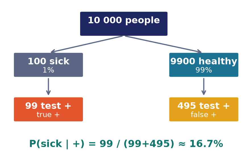
Natural-frequency cross-check. Abandon fractions and imagine a concrete cohort of people. This “confusion matrix” is exactly the contingency table used to evaluate classifiers in machine learning:
| Test | Test | Row total | |
|---|---|---|---|
| Diseased () | (true pos.) | (false neg.) | |
| Healthy () | (false pos.) | (true neg.) | |
| Column total |
Of the people who test positive, only are truly ill, so — identical to Bayes, and far easier to feel. The odds form gives the same answer in one line: prior odds , likelihood ratio , posterior odds , hence posterior probability .
CS / ML connection. In classifier terms the table’s quantities are named: recall (sensitivity) , and precision . A spam filter faces the same arithmetic — a rare event (a genuine phishing mail) with an imperfect detector — and a naive Bayes classifier is literally Bayes’ theorem applied under a simplifying independence assumption on the features (words). Base-rate neglect is the human bug that Bayesian reasoning fixes.
13.13 The birthday problem
In a room of people, how likely is it that two share a birthday? The answer is famously larger than intuition suggests, and it is the exact model of hash collisions.
Setup. Assume equally likely birthdays, independent across people (ignore leap days and twins). The sample space of birthday assignments has equally likely elements. Let “some two of the people share a birthday.” Compute the complement “all birthdays are distinct” — far easier to count.
Derivation. Assigning distinct birthdays is an ordered selection of days from without repetition, i.e. a -permutation with :
Therefore . Tabulating:
| 10 | 0.8831 | 0.1169 |
| 20 | 0.5886 | 0.4114 |
| 23 | 0.4927 | 0.5073 |
| 30 | 0.2937 | 0.7063 |
| 40 | 0.1088 | 0.8912 |
| 50 | 0.0296 | 0.9704 |
| 70 | 0.0008 | 0.9992 |
At the probability of a shared birthday first exceeds — only people, not the (half of ) that intuition often guesses. By a match is virtually certain.
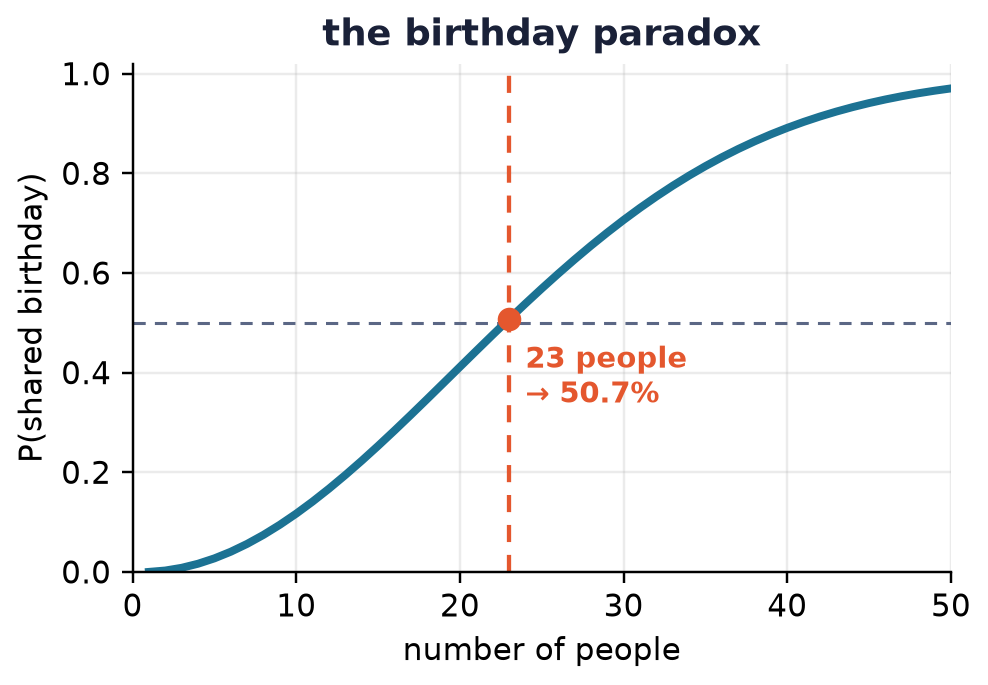
Why so few? A shared birthday needs only some pair to coincide, and people form pairs — a quantity that grows like . For that is pairs, already comparable to . The standard approximation makes this precise: using ,
For : , and , so — matching the exact .
CS connection (hash collisions and the birthday attack). Replace by the number of hash buckets (or possible hash values). The same computation shows that once about items have been hashed, a collision becomes more likely than not. This is why a hash function with a -bit output () offers only about collision resistance, and why the birthday attack forces cryptographic hash lengths to be doubled: to resist collisions at the level, one needs a -bit hash. The birthday problem is thus a load-bearing calculation in the design of hash tables and cryptographic digests.
13.14 The Monty Hall problem
A game show has three doors: behind one is a car, behind the other two are goats. You pick a door. The host — who knows what is behind each door — opens a different door, always revealing a goat, and offers you the chance to switch to the remaining unopened door. Should you switch?
State the rules precisely (they matter). The standard problem assumes:
- the car is equally likely behind any door;
- the host always opens a door you did not pick and always reveals a goat;
- if your initial pick hides the car (so the host has two goat doors to choose from), the host picks between them uniformly at random.
Under these rules the answer is that switching wins with probability , staying only . Two independent arguments confirm it.
Argument 1 (enumeration on the initial pick). Your first choice is right (car) with probability and wrong (goat) with probability .
- If your first pick was the car (): the other unopened door hides a goat, so switching loses.
- If your first pick was a goat (): the host is forced to reveal the other goat, so the remaining unopened door hides the car, and switching wins.
Hence .
Argument 2 (Bayes). Say you pick door 1 and the host opens door 3. Let “car behind door ” (priors each) and “host opens door 3.” The likelihoods encode the rules:
| Hypothesis | reason | |
|---|---|---|
| (your door) | host free to open 2 or 3, chooses randomly | |
| host cannot open 1 (yours) or 2 (car) → must open 3 | ||
| host never opens the car’s door |
By total probability . Then Bayes gives
Staying keeps door 1 with win probability ; switching moves to door 2 with win probability . ∎
Why intuition fails (the crucial point). The two remaining doors are not symmetric, so “it’s now 50-50” is wrong. The host’s action carries information: when your first pick was a goat (probability ), the host is forced to expose the only other goat, effectively pointing at the car. Switching converts your initial chance of being wrong into a chance of winning. If instead the host opened a door at random and merely happened to reveal a goat, the information would be different and the odds would indeed become — which is why stating the rules is not pedantry.
13.15 Random variables and expectation
Often we care not about which outcome occurs but about a number attached to it — the sum of two dice, the number of collisions in a hash table, the running time of a randomized algorithm.
Definition (random variable). A random variable on a sample space is a function assigning a real number to each outcome. For discrete its probability mass function is ; the masses are non-negative and sum to over the possible values.
Example. For one die, has for . For two dice, “sum” is a random variable with the mass function tabulated in Problem 2.
Indicator variables. The indicator of an event is if and otherwise. It converts an event into a -valued random variable and is the bridge between events and expectations.
Definition (expectation). The expected value (mean) of a discrete random variable is the probability-weighted average of its values,
It is the “long-run average” the value of approaches when the experiment is repeated many times (this is what the law of large numbers guarantees).
Example (one die). . The mean is not itself an attainable value — expectation is an average, not a prediction of any single roll.
Example (indicator). . The expected value of an indicator is just the probability of its event — the identity that makes the next theorem so useful.
Theorem (linearity of expectation). For any random variables on the same finite and constants ,
Crucially, this holds whether or not and are independent.
Proof. Using the outcome-sum form of expectation and rearranging a finite sum,
The only facts used are the distributive law and that a finite sum can be split — no independence anywhere. ∎
Example (sum of two dice, via linearity). Let be the two dice. Then , instantly — no need to weight the sum-values by the table in Problem 2 (though doing so also gives ). Linearity turns a messy convolution into one line.
Example (expected number of birthday matches). Among people, let count the pairs sharing a birthday. Writing , where indicates that persons match, linearity and give
For , — the very exponent that appeared in the birthday approximation, now explained: matches become likely exactly when the expected number of matching pairs reaches order . (Note the pair-events are not independent, yet linearity still applies — its great strength.)
Bernoulli and binomial. An event with defines a Bernoulli variable with . Repeating independent Bernoulli trials, the count of successes is binomial, , and writing gives by linearity
For example, in fair coin flips the expected number of heads is .
Variance and standard deviation
The mean alone does not capture spread. The variance of is the expected squared deviation from the mean,
and the standard deviation is in the same units as . For the single die, and . Two handy rules: , and for independent , .
For a dataset — the descriptive-statistics view used in Lab 7 — the same formula with equal weights gives the population mean, variance, and standard deviation
the sample variance divides by instead of (an unbiased estimate when the data are a sample, not the whole population). Variance also controls how fast averages converge (Chebyshev’s inequality, concentration bounds) — a theme of the next course, and the reason randomized algorithms are reliably fast, not merely fast on average.
A short history
Games of chance are ancient, but their mathematics is not. Gerolamo Cardano (c. 1564) wrote the first analysis of dice odds. The subject proper was born in 1654 in the correspondence between Blaise Pascal and Pierre de Fermat, prompted by exactly the kind of gambling puzzle de Méré posed above. Christiaan Huygens wrote the first textbook (1657); Jacob Bernoulli proved the first law of large numbers (published 1713), rigorously linking probability to long-run frequency; Thomas Bayes’ essay on inverse probability appeared posthumously (1763); and Pierre-Simon Laplace systematized the classical definition around 1812. The modern axiomatic foundation — the three axioms of this lecture, freeing probability from any reliance on symmetry or frequency — was laid by Andrey Kolmogorov in 1933, and it is his framework we have used throughout.
Chapter summary
- A random experiment has a sample space of elementary outcomes; an event is a subset . Events are sets, so the union/intersection/ complement algebra and De Morgan’s laws of Lectures 1–2 transfer verbatim (the event–set dictionary).
- Event types: certain (), impossible (), compatible vs. incompatible (), complementary , a complete group (partition, cf. Lecture 3), and independent vs. dependent.
- Classical probability for equally likely outcomes reduces probability to counting; the statistical view estimates by relative frequency (law of large numbers) when symmetry is unavailable.
- Combinatorics. Multiplication principle permutations , arrangements , combinations (derived via ); Pascal’s identity .
- Kolmogorov’s axioms: , , additivity over incompatible events — from which we proved , , , monotonicity, the addition rule (a probabilistic inclusion–exclusion), its three-event form, and Boole’s inequality (union bound).
- Conditional probability shrinks the sample space to ; the multiplication rule and its chain rule generalization follow.
- Independence: , equivalently . Incompatible events of positive probability are provably dependent.
- Law of total probability (proved via a partition) and Bayes’ theorem (proved from it) turn priors + likelihoods into posteriors; the odds form multiplies prior odds by the likelihood ratio.
- Three set pieces: the birthday problem (; models hash/birthday-attack collisions at ), Monty Hall (switch to win ), and the medical-test Bayes calculation (; base-rate neglect).
- Random variables and expectation ; linearity of expectation holds without independence; a binomial count has .
Exercises
Warm-up
- Roll one fair die. Write , and as subsets the events “odd,” “at least .” Compute , , , and verify the addition rule.
- Give for tossing three distinguishable coins and its size. Find the probability of exactly two heads.
- Explain in one sentence each the difference between (a) incompatible and independent events, and (b) and .
- A committee of is chosen from people. How many committees are possible? If instead the four take distinct roles (chair, secretary, treasurer, webmaster), how many role-assignments are possible?
- From a standard deck, find , , and .
Standard
- (Derive a rule.) Using only Kolmogorov’s axioms, prove , and state where you use additivity.
- Two fair dice are rolled. Find , , and .
- An urn has red, green, blue balls; draw without replacement. Find the probability of (a) all red, (b) one of each colour, (c) at least one blue.
- A box has good and defective chips; draw without replacement. Find the probability both are good, first via the multiplication rule and again via combinations, and confirm the answers agree.
- Cards: two are drawn without replacement. Find and .
- (Total probability.) Factory lines I, II, III make of output with defect rates . Find the probability a random item is defective.
- (Bayes.) For Exercise 11, a random item is found defective. Which line most probably produced it? Give all three posterior probabilities.
- A test for a condition present in of people has sensitivity and false-positive rate . Find by Bayes, and cross-check with a natural-frequency table of people.
- Show, using indicators and linearity, that the expected number of sixes in rolls of a fair die is . Evaluate for .
Challenge
- (Birthday variant.) In a room of people, let “someone shares your birthday.” Show and find the smallest making . Explain why this is far larger than .
- (Monty Hall, doors.) Generalize Monty Hall to doors (one car), where after your pick the host opens exactly one goat door and offers a single switch. Show switching wins with probability for , and compare staying’s .
- (Inclusion–exclusion.) Three fair dice are rolled. Using the three-event addition rule, find the probability that at least one die shows a six.
- (De Méré, generalized.) For how many rolls of a single die does first exceed ? Justify with the complement rule.
- (Prosecutor’s fallacy.) A DNA test declares a match with probability in for a random innocent person. In a database of million innocent people, a match is found. Use the union bound (or expectation) to explain why “one in a million” does not mean the matched person is almost surely guilty.
- (Pairwise vs. mutual independence.) Toss two fair coins; let “first is heads,” “second is heads,” “the two coins agree.” Show are pairwise independent but not mutually independent.
Selected answers & hints
- 1. ; ; , so , so ; check . ✓
- 2. ; exactly two heads is outcomes, probability .
- 4. Committees: . Distinct roles: .
- 5. ; ; red-or-queen .
- 7. ; ; sum is odd, so .
- 8. Total . (a) . (b) . (c) complement (no blue) , so .
- 9. ; and . ✓
- 11. .
- 12. Posteriors each term over : line I , II , III . Lines I and III tie as most probable.
- 13. ; . Cohort of : affected → true positives; unaffected → false positives; . ✓
- 15. Each other person misses your birthday with probability , independently, so . Solve : , so . It is huge compared to because only comparisons target your fixed day, versus comparisons among all pairs in the classic problem.
- 17. ; the three-event inclusion–exclusion gives , agreeing.
- 18. , so (matching De Méré’s Bet A, ).
- 20. ; pairwise , , likewise . But , so not mutually independent.
Further reading
- K. H. Rosen, Discrete Mathematics and Its Applications — chapters on Discrete Probability and Counting (the multiplication principle, permutations/combinations, Bayes’ theorem, and expected value are developed at this level).
- S. Ross, A First Course in Probability — a fuller, rigorous treatment of axioms, conditional probability, independence, and random variables.
- C. M. Grinstead and J. L. Snell, Introduction to Probability (freely available) — excellent worked problems, including Monty Hall and the birthday problem.
- For the algorithmic side: M. Mitzenmacher and E. Upfal, Probability and Computing — the union bound, hashing, and randomized algorithms in depth.